Adult Mosquito Models • ramp.xds

library(ramp.xds)
library(viridisLite)

ramp.xds includes five modules describing adult mosquito ecology, behavior, and infection dynamics. They were included to illustrate some of the core concepts and design features of ramp.xds, particularly the issue of extensibility in non-autonomous systems, where we are concerned about combining the effects of exogenous forcing and vector control to develop models that can regard malaria transmission as a changing baseline that has been modified by control.

ramp.library includes an expanded set of models for adult mosquitoes, including models with mosquito chronological or reproductive age, and behavioral state models (see MYZ-Overview).

The dynamical terms required by $\cal MYZ$ models are:

Lambda or $\Lambda$ - the emergence rates of adult mosquitoes in the patches
kappa or $\kappa$ - net infectiousness (NI), the probability a mosquito becomes infected after blood feeding on a human. The dynamical terms output by $\cal MYZ$ models are:
F_fqZ outputs the number of bites by infectious mosquitoes, per patch, per day
F_fqM outputs the number of bites by mosquitoes, per patch, per day
F_eggs outputs the number of eggs laid by mosquitoes, per patch, per day

In this vignette, we discuss the challenge of extensibility, in particular, the challenges of modeling malaria transmission by mosquitoes as a changing baseline that has been modified by vector control.

The models in ramp.xds were included for several reasons:

They serve as an important set of models to test the software;
They illustrate some important basic features of ramp.xds design princples (see Nimble Model Building and Scalable Complexity).

Basic Models

All five models use a common set of parameters:

$\tau$ the parasite’s extrinsic incubation period (EIP)
$f$ the patch-specific overall feeding rates
$q$ the patch-specific human fraction
$g$ the patch-specific mortality rate
$\sigma$ the patch-specific emigration rate
$\mu$ patch-specific mortality associated with emigration
$\nu$ patch-specific egg-laying rates
$\cal K$ a dispersal matrix

ramp.xds there are several versions of basic models for mosquito infection dynamics. These models make similar assumptions about mosquito ecology and infection dynamics. (The equations are in the documentation for The four models are

GeRM. This implements a fully generalized, non-autonomous version of the Ross-Macdonald model. The base model was the delay differential equation Ross-Macdonald model presented by from Aron & May (1982). It has been extended to include generalized exogenous forcing and egg laying, as described by Wu SL, et al. (2023): the baseline values of bionomic parameters (generically $x$ ) are evaluated by a function $F_x(t,V,\mbox{par}_x).$ The equations were formulated using novel built-in numerical algorithms to compute survival and dispersal through a time-varying extrinsic incubation period.

GeRM <- xds_setup(Xname = "trivial", Xopts = list(kappa = .1),
                MYZname = "GeRM", MYZopts = list(Y=0, Z=0))

GeRM <- xds_solve(GeRM, Tmax=80)

rm - This version of the Ross-Macdonald model, as a system of delay differential equations, that follows the formulation by Aron & May (1982), which allows for mosquito population density to fluctuate, forced by emergence $\Lambda(t)$ . The model has been included as a teaching model with the warning that it is not extensible: the parameters are assigned static values, so it can not accommodate exogenous forcing of the bionomic parameters.

macdonald <- xds_setup(Xname = "trivial", Xopts = list(kappa = .1),
                MYZname = "macdonald", MYZopts = list(Y=0, Z=0))

macdonald <- xds_solve(macdonald, Tmax=80)



+ [**`basicM`**](https://dd-harp.github.io/ramp.xds/reference/dMYZdt.basicM.html) is based on **`GeRM`,** but it lacks variables describing infected or infectious mosquitoes. 


``` r
basicM <- xds_setup(Xname = "trivial", Xopts = list(kappa = .1), 
                    MYZname = "basicM")

basicM <- xds_solve(basicM, Tmax=80)

si is a basic SI compartmental model for infection in mosquitoes that was set up to accommodate a static baseline with exogenous forcing by vector control. It assumes that the density of infectious mosquitoes is the density of infected mosquitoes modified by survival and dispersal through an EIP, computed with present parameters $Z = e^{-\Omega \tau} \cdot Y.$

SI <- xds_setup(Xname = "trivial", Xopts = list(kappa = .1), 
                MYZname = "SI", MYZopts = list(Y=0))

SI <- xds_solve(SI, Tmax=80)

SEI is a standard SEI compartmental model that is fully parameterized for exogenous forcing.

SEI <- xds_setup(Xname = "trivial", Xopts = list(kappa = .1), 
                 MYZname = "SEI", MYZopts = list(Y=0, Z=0))

SEI <- xds_solve(SEI, Tmax=80)

Ecology

The ecology for basicM and si and SEI and rm is identical. Let $M$ denote the density of adult mosquitoes, $\Lambda(t)$ the emergence rate of adult mosquitoes from aquatic habitats, and $g$ the adult mosquito mortality rate. Mosquito population density is described by an equation:

$\frac{dM}{dt} = \Lambda(t) - g M$ If $n_p>1$ then $M$ is a vector and we formulate a demographic matrix as described in Spatial Dynamics of Malaria Transmission (2023) PLoS Computational Biology. The models have four parameter families:

$g$ the patch-specific daily mortality rates (the probability of surviving one day is $p = e^{-g}$
$\sigma$ is a patch-specific daily emigration rate
$\mu$ is the a patch-specific proportion lost through migration
$\cal K$ is a mosquito dispersal matrix

$$\Omega = \mbox{diag}\left(g\right) + \left[ \mbox{diag}\left(1-\mu\right) - {\cal K} \right] \cdot \mbox{diag}\left(\sigma\right)$$ Note that if $n_p=1$ , then $\Omega = g$ . This gives us the more general formulation:

$\frac{dM}{dt} = \Lambda(t) - \Omega \cdot M$

If $\Lambda$ is constant, then the equation has a steady state:

$\bar M = \Omega^{-1} \cdot \Lambda$

xds_plot_M(basicM)
xds_plot_M(SI, add=TRUE, clrs="darkred")
xds_plot_M(SEI, add=TRUE, clrs = "darkblue")
xds_plot_M(macdonald, add=TRUE, clrs = "orange")
xds_plot_M(GeRM, add=TRUE, clrs = "darkgreen")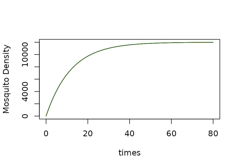

Infection

The infection dynamics for si and SEI and rm are identical. (The model basicM does not define a variable $Y$ ).

The dynamics of infection depend on a quantity that we will call $\kappa(t)$ denoting the net infectiousness (NI) of humans, or the probability a mosquito becomes infected after blood feeding on a human. Let $f$ denote the overall blood feeding rate, and let $q$ denote the fraction of blood meals on humans (a.k.a the human fraction). Let $Y$ denote the density of mosquitoes that are infected with parasites, and its dynamics are described by:

$\frac{dY}{dt} = fq\kappa(M-Y) - \Omega \cdot Y$

xds_plot_Y(SI, llty=1, clrs="darkred")
xds_plot_Y(SEI, add=TRUE, llty=2, clrs = "darkblue")
xds_plot_Y(macdonald, add=TRUE, llty=3, clrs = "orange")
xds_plot_Y(GeRM, add=TRUE, llty=3, clrs = "darkgreen")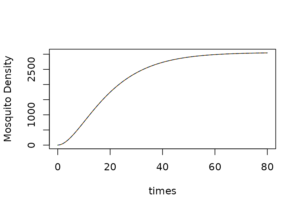

If $M$ and $\kappa$ have reached the steady state, then the fraction of infected mosquitoes, $y=Y/M$ is given by:

$y = \frac{fq\kappa}{g+fq\kappa}$

and the fraction of infectious mosquitoes (i.e. with sporozoites in their salivary glands), is called the sporozoite rate,

$z = e^{-g\tau} \frac{fq\kappa}{g+fq\kappa}$

Infectiousness

Let $Z$ denote the density of mosquitoes that have sporozoites in their salivary glands, and let $\tau$ denote the time elapsed between the blood meal that infects a mosquito and the point in time when a surviving mosquito has sporozoites in its salivary glands. The probability a mosquito has survived $\tau$ days is $e^{-g\tau}$ , and we let a subscripted $\tau$ denote the value of a variable at time $t-\tau.$

In rm the density of infectious mosquitoes is modeled by:

$\frac{dZ}{dt} = e^{-g \tau} fq\kappa_\tau(M_\tau-Y_\tau) - gZ$

In the si model, the density of infectious mosquitoes has ignored the delay, but it discounts biting by the fraction that would survive (and disperse) through the EIP. To put it another way si and rm would have the same steady state if autonomous model.

$Z = e^{-\Omega \tau}\cdot Y$

In the si model, the density of infectious mosquitoes has ignored the delay, but it discounts biting by the fraction that would survive (and disperse) through the EIP.

$dZ/dt = (Y-Z)/\tau- \Omega \cdot Z$

xds_plot_Z(SEI, llty=1, clrs="darkblue")
xds_plot_Z(SI, add=TRUE, clrs = "darkred")
xds_plot_Z(macdonald, add=TRUE, clrs = "orange")
xds_plot_Z(GeRM, add=TRUE, llty=3, clrs = "darkgreen")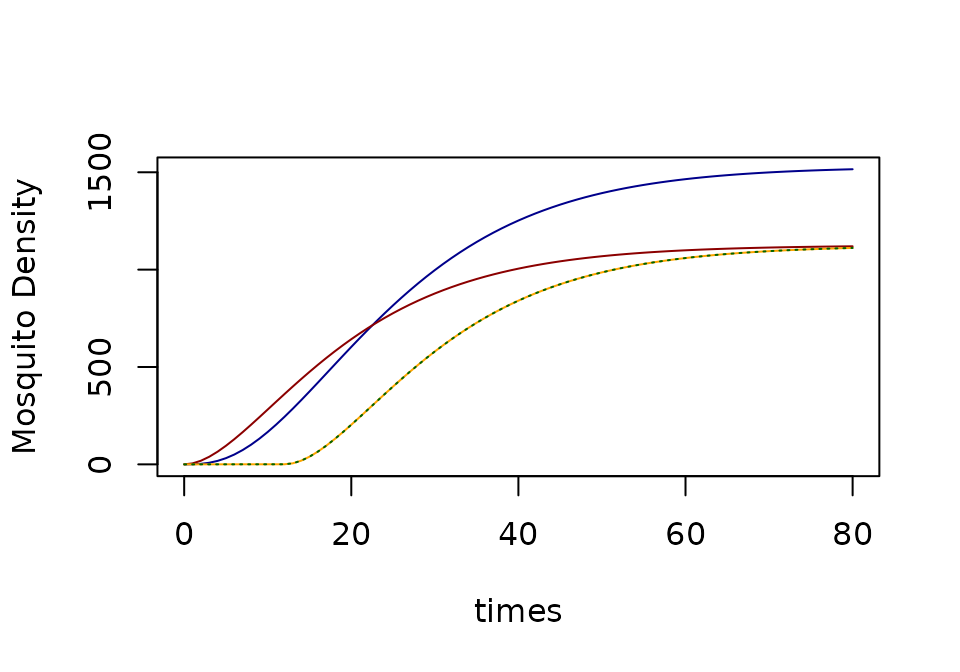

xds_plot_Z_fracs(SEI, clrs="darkblue")
xds_plot_Z_fracs(macdonald,  add=T, clrs = "orange")
xds_plot_Z_fracs(SEI, add=T, clrs="darkblue")
xds_plot_Z_fracs(SI, add=T,  clrs = "darkred")
xds_plot_Z_fracs(GeRM, add=TRUE, llty=3, clrs = "darkgreen")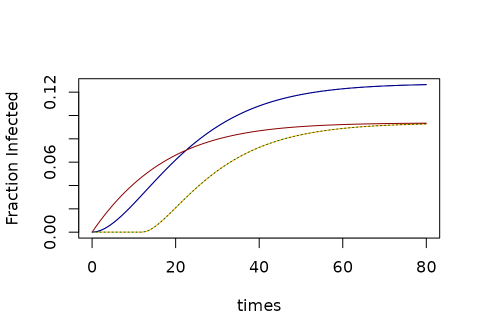

This is equivalent to Macdonald’s formula.

In ramp.xds this set of equations is implemented. This sets up and solves a model with $\kappa$ and $\Lambda$ passed as constant values, and a human population density of $H=10.$

macdonald = xds_setup(Xname = "trivial", Xopts=list(kappa=0.1), Lname = "trivial", Lopts = list(Lambda=5), HPop=10)
macdonald = xds_solve(macdonald, Tmax=100)

xds_plot_M(macdonald)
xds_plot_Y(macdonald, add=TRUE)
xds_plot_Z(macdonald, add=TRUE)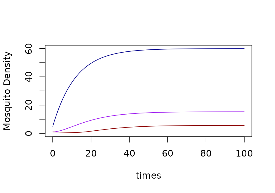

Macdonald’s Formula

If we wanted to replicate Macdonald’s equations, we would let $a=fq$ , $p = e^{-g}$ or equivalently $g = -\ln p$ , $\kappa = x,$ and $n=\tau$ so:

$e^{-g\tau} \frac{fq\kappa}{g+fq\kappa} = p^n \frac{ax}{ax - \log_{e}p}$

Lo = list(season = function(t){1+sin(2*pi*t/365)}, 
          trend = function(t){exp(-t/1000)}, 
          Lambda =5)
macdonald = xds_setup(Xname = "trivial", Xopts = list(kappa=0.1), HPop=10,
               Lname = "trivial", Lopts = Lo)
macdonald <- xds_solve(macdonald, 3680, dt=10)

xds_plot_M(macdonald)

Exogenous Forcing

A challenge for these models was to compute the bionomic parameters as a baseline that was modified by control. A challenge for making software that was extensible was how to accommodate various ways.