basicL

The basicL_xde competition aquatic mosquito model fulfills the generic interface of the aquatic mosquito component. It has a single compartment “larvae” for each aquatic habitat, and mosquitoes in that aquatic habitat suffer density-independent and dependent mortality, and mature at some rate $ψ$ .

Differential Equations

Given $Λ$ and some egg laying rate from the adult mosquito population we could formulate and solve a dynamical model of aquatic mosquitoes to give that emergence rate. However, in the example here we will simply use a trivial-based (forced) emergence model, so that $Λ$ completely specifies the aquatic mosquitoes.

The simplest model of aquatic (immature) mosquito dynamics with negative feedback (density dependence) is:

$\dot{L} = η - (ψ + ϕ + θ L) L$

Because the equations allow the number of larval habitats $l$ to differ from $p$ , in general the emergence rate is given by:

$Λ = N \cdot α$

Where $N$ is a $p \times l$ matrix and $α$ is a length $l$ column vector given as:

$α = ψ L$

Equilibrium solutions

In general, if we know the value of $Λ$ at equilibrium we can solve for $L$ directly by using the above two equations. Then we can consider $θ$ , the strength of density dependence to be unknown and solve such that:

$θ = (η - ψ L - ϕ L) / L^{2}$

Example

library(ramp.xds)
library(deSolve)
library(data.table)
library(ggplot2)

The long way

Here we run a simple example with 3 aquatic habitats at equilibrium. We use ramp.xds::make_parameters_L_basicL_xde to set up parameters. Please note that this only runs the aquatic mosquito component and that most users should read our fully worked example to run a full simulation.

nHabitats <- 3
nPatches=nHabitats
membership=1:nPatches
params <- make_xds_template("ode", "aquatic", nPatches, membership)

alpha <- c(10, 50, 20)
eta <- c(250, 500, 170)
psi <- 1/10
phi <- 1/12
L <- alpha/psi
theta <- (eta - psi*L - phi*L)/(L^2)
Lo = list(eta=eta, psi=psi, phi=phi, theta=theta, L=L)
MYZo = list(MYZm <- eta)

#params$Xpar[[1]]=list() 
#class(params$Xpar[[1]]) <- "trivial"
#params$MYZpar[[1]]=list() 

params$eggs_laid = list() 
params$eggs_laid[[1]] = eta 
F_eta = function(t, pars){
  pars$eggs_laid[[1]]
}

params = setup_Lpar("basicL", params, 1, Lo)
params = setup_Linits(params, 1, Lo)
params = setup_MYZpar("trivial", params, 1, MYZo)

params = make_indices(params)

xDE_aquatic = function(t, y, pars, F_eta) {
  pars$eggs_laid[[1]] <- F_eta(t, pars)
  dL <- dLdt(t, y, pars, 1)
  return(list(c(dL)))
}

y0 <- get_inits(params) 

out <- deSolve::ode(y = as.vector(unlist(y0)), times = seq(0,50,by=10), xDE_aquatic, parms = params, method = 'lsoda', F_eta = F_eta) 
out1 <- out

colnames(out)[params$L_ix+1] <- paste0('L_', 1:params$nHabitats)

out <- as.data.table(out)
out <- melt(out, id.vars = 'time')
out[, c("Component", "Patch") := tstrsplit(variable, '_', fixed = TRUE)]
out[, variable := NULL]

ggplot(data = out, mapping = aes(x = time, y = value, color = Patch)) +
  geom_line() +
  theme_bw()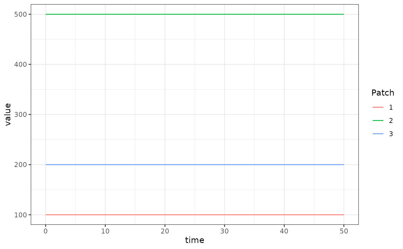

Using Setup

The function xds_setup_aquatic sets up a model that includes only aquatic dynamics, and it is solved using xds_solve.aqua. The setup functions are simpler than xds_setup and come with constrained choices. The user can configure any aquatic model (trivial wouldn’t make much sense), and it uses trivial to force egg laying.

We configure the aquatic model: Lo is a list with the parameter values attached.

Lo = list(
  psi = 1/10, 
  phi = 1/12
)
alpha = c(10, 50, 20)
Lo$L = with(Lo, alpha/psi) 
Lo$theta = with(Lo, (eta - psi*L - phi*L)/(L^2))

We use the MYZ model trivial to configure egg laying.

Mo = list(MYZm = c(250, 500, 170))

xds_setup_aquatic(nHabitats=3, Lname = "basicL", Lopts = Lo, MYZopts = Mo) -> aqbasicL_xde
xds_solve(aqbasicL_xde, Tmax=50, dt=10)$output$orbits$deout -> out2
sum(abs(out1-out2)) == 0
#> [1] TRUE

A Basic Model for Immature Mosquitoes

Differential Equations

Equilibrium solutions

Example

The long way

Using Setup