Macdonald's Model
A Delay Differential Equation for Adult Mosquito Infection Dynamics
Source:vignettes/adult_RM.Rmd
adult_RM.RmdThis module called macdonald was included in
ramp.xds for historical reasons. In this
form, the model is difficult to extend because of problems formulating
the delay. The model, as presented here, has fixed parameter values. It
can not be extended with forcing. To address these problems, we
have developed a fully extensible delay differential equation model that
extends macdonald, the generalized, non-autonomous
Ross-Macdonald module GeRM.
Differential Equations
Macdonald’s Equations
Macdonald’s model for the sporozoite rate, published in 19521 has played an important role in studies of malaria. Later that same year, Macdonald introduced a formula for the basic reproductive rate, now called \(R_0.\)2 Macdonald gives credit to his colleague Armitage for the mathematics. Armitage’s paper would be published the next year,3 but that paper does not present the model as a system of differential equations.
A simple system of differential equations that is consistent with Macdonald’s model for the sporozoite rate has three parameters and one term:
the human blood feeding rate, \(a\)
the extrinsic incubation period, \(\tau\)
the mosquito death rate, \(g\); or the probability of surviving one day, \(p=e^{-g}\), so \(g=-\ln p\)
the fraction of bites on humans that infect a mosquito, \(\kappa\)
Let \(y\) denote the fraction of
mosquitoes that are infected. The dynamics are given by: \[\frac{dy}{dt} = a \kappa (1-y) - g y\] Let
\(z\) denote the fraction of mosquitoes
that are infectious. The model is a delay differential equation. Let
\(y_\tau\) denote the value of \(y\) at time \(t-\tau.\) If the parameters and terms are
constant, then:
\[\frac{dz}{dt} = e^{-g\tau} a \kappa
(1-y_\tau) - g z\] The model has a steady state for the fraction
infected: \[\bar y = \frac{a \kappa} {a
\kappa + g}\] The fraction infectious, also called the sporozoite
rate, is \[\bar z = \frac{a \kappa} {a \kappa
+ g}e^{-g\tau}.\] Macdonald used \(p\) so his formula was: \[\bar z = \frac{a \kappa} {a \kappa -\ln
p}e^{-p\tau}\]
To generate the formula for \(R_0,\) Macdonald introduces another variable and three additional parameters:
the ratio of mosquitoes to humans, \(m\)
the rate infections clear, \(r\)
the fraction of infectious bites that infect a human, \(b\)
The fraction of infected and infectious humans, \(x,\) is given by the equation:
\[\frac{dx}{dt} = m a z (1-y) - r x\] and the model assumes that \(\kappa = x.\) The formula for \(R_0\) in this system is: \[R_0 = \frac{m b a^2}{gr} e^{-g\tau} = \frac{m b a^2}{(-\ln p)r} e^{-p\tau}\] In this form, the model is difficult to use or extend.
Aron & May
The mosquito module in ramp.xds called
macdonald is based on a model first published in 1982 by
Joan Aron and Robert May4. It includes state variables for total
mosquito density \(M\), infected
mosquito density \(Y\), and infectious
mosquito density \(Z\). In this model,
the blood feeding rate is split into an overall blood feeding rate,
\(f\), and the human fraction, \(q\) such that \[a=fq.\] The Aron & May’s equations
are: \[\begin{array}{rl}
\frac{dM}{dt} &= \Lambda(t) - g M \\
\frac{dY}{dt} &= fq\kappa(M-Y) - g Y \\
\frac{dZ}{dt} &= e^{-g\tau}fq\kappa_\tau(M_\tau-Y_\tau) - g Z \\
\end{array}\]
Delay Differential Equations
The module called macdonald has been extended beyond the
Aron & May formulation to include spatial dynamics and parity. To
formulate the spatial model, a spatial domain is sub-divided into a set
of patches. Variable and parameter names do not change, but they can now
represent vectors of length \(n_p.\) To
formulate the demographic matrix, denoted \(\Omega,\) that describes mosquito
mortality, emigration, and other loss from the system. We let \(\sigma\) denote the emigration rate and
\(\cal K\) the mosquito dispersal
matrix. We also introduce a parameter, \(\mu\) to model the fraction of mosquitoes
that are lost to emigration from each patch. \[\Omega = \mbox{diag} \left(g\right) +
\left(\mbox{diag} \left(1-\mu\right) - \cal K\right) \cdot \mbox{diag}
\left(\sigma\right)
\]
Dynamics
\[\begin{array}{rl} \dot{M} & = \Lambda - \Omega\cdot M \\ \dot{P} & = \mbox{diag}(f) \cdot (M-P) - \Omega \cdot P\\ \dot{Y} & = \mbox{diag}(fq\kappa) \cdot (M-Y) - \Omega \cdot Y \\ \dot{Z} & = \dot{Z} = e^{-\Omega \tau} \cdot \mbox{diag}(fq\kappa_{t-\tau}) \cdot (M_{t-\tau}-Y_{t-\tau}) - \Omega \cdot Z \end{array} \]
Ordinary Differential Equations
We note that the module SI provides a reasonably simple
approximating model that has no delay, but in computing \(fqZ,\) it includes mortality and dispersal
that would have occurred during the EIP: \[
Z = e^{-\Omega \tau} \cdot Y
\] The implementation of SI is similar in spirit to
the simple model presented in Smith & McKenzie (2004)5. in that mortality and
dispersal over the EIP is accounted for, but the time lag is not. While
transient dynamics of the ODE model will not equal the DDE model, they
have the same equilibrium values, and so for numerical work requiring
finding equilibrium points, the faster ODE model can be safely
substituted.
Equilibrium solutions
There are two logical ways to begin solving the non-trivial equilibrium. The first assumes \(\Lambda\) is known, which implies good knowledge of mosquito ecology. The second assumes \(Z\) is known, which implies knowledge of the biting rate on the human population. We show both below.
Starting with \(\Lambda\)
Given \(\Lambda\) we can solve:
\[ M = \Omega^{-1} \cdot \Lambda \] Then given \(M\) we set \(\dot{Y}\) to zero and factor out \(Y\) to get:
\[ Y = (\mbox{diag}(fq\kappa) + \Omega)^{-1} \cdot \mbox{diag}(fq\kappa) \cdot M \] We set \(\dot{Z}\) to zero to get:
\[ Z = \Omega^{-1} \cdot e^{-\Omega \tau} \cdot \mbox{diag}(fq\kappa) \cdot (M-Y) \]
Because the dynamics of \(P\) are independent of the infection dynamics, we can solve it given \(M\) as:
\[ P = (\Omega + \mbox{diag}(f))^{-1} \cdot \mbox{diag}(f) \cdot M \]
Starting with \(Z\)
It is more common that we start from an estimate of \(Z\), perhaps derived from an estimated EIR (entomological inoculation rate). Given \(Z\), we can calculate the other state variables and \(\Lambda\). For numerical implementation, note that \((e^{-\Omega\tau})^{-1} = e^{\Omega\tau}\).
\[ M-Y = \mbox{diag}(1/fq\kappa) \cdot (e^{-\Omega\tau})^{-1} \cdot \Omega \cdot Z \]
\[ Y = \Omega^{-1} \cdot \mbox{diag}(fq\kappa) \cdot (M-Y) \]
\[ M = (M - Y) + Y \]
\[ \Lambda = \Omega \cdot M \] We can use the same equation for \(P\) as above.
Example
Here we show an example of starting and solving a model at equilibrium. Please note that this only runs this adult mosquito model and that most users should read our fully worked example to run a full simulation.
Ross-Macdonald
\[ \begin{array}{rl} \frac{\textstyle{dy}}{\textstyle{dt}} & = a \kappa \left(1 -y \right) - g y \\ \frac{\textstyle{dz}}{\textstyle{dt}} & = e^{-g\tau} q \kappa_\tau \left[1 - y_\tau \right] - g z \end{array} \]
The long way
Here we set up some parameters for a simulation with 3 patches.
HPop = rep(1, 3)
nPatches <- 3
f <- rep(0.3, nPatches)
q <- rep(0.9, nPatches)
g <- rep(1/20, nPatches)
sigma <- rep(1/10, nPatches)
mu <- rep(0, nPatches)
eip <- 12
nu <- 1/2
eggsPerBatch <- 30
MYo = list(f=f,q=q,g=g,sigma=sigma,mu=mu,eip=eip,nu=nu,eggsPerBatch=eggsPerBatch)
K_matrix <- diag(-1, nPatches)
K_matrix[2:3, 1] <- c(0.2, 0.8)
K_matrix[c(1,3), 2] <- c(0.5, 0.5)
K_matrix[1:2, 3] <- c(0.7, 0.3)

Omega <- compute_Omega_xde(g, sigma, mu, K_matrix)
Upsilon <- expm::expm(-Omega * eip)
Now we set up the parameter environment with the correct class using
ramp.xds::make_parameters_MY_RM_xde, noting that we will be
solving as an ode.
Now we set the values of \(\kappa\) and \(\Lambda\) and solve for the equilibrium values.
Omega_inv <- solve(Omega)
M_eq <- as.vector(Omega_inv %*% Lambda)
P_eq <- as.vector(solve(diag(f, nPatches) + Omega) %*% diag(f, nPatches) %*% M_eq)
Y_eq <- as.vector(solve(diag(f*q*kappa) + Omega) %*% diag(f*q*kappa) %*% M_eq)
Z_eq <- as.vector(Omega_inv %*% Upsilon %*% diag(f*q*kappa) %*% (M_eq - Y_eq))
MYo$M=M_eq
MYo$P=P_eq
MYo$Y=Y_eq
MYo$Z=Z_eq
We use ramp.xds::make_inits_MY_RM_xde to store the
initial values. These equations have been implemented to compute \(\Upsilon\) dynamically, so we attach
Upsilon as initial values:
params <- make_xds_object_template("dde", "mosy", nPatches, 1:3, 1:3)
params <- setup_MY_obj("macdonald", params, 1, MYo)
params <- setup_MY_inits(params, 1, MYo)
params <- setup_XH_obj("trivial", params, 1, Xo)
params <- setup_XH_inits(params, HPop, 1)
params <- setup_L_obj("trivial", params, 1, Lo)
params <- setup_L_inits(params, 1, Lo)
We set the indices with ramp.xds::make_indices.
params = make_indices(params)
params <- change_K_matrix(K_matrix, params, "0", 1)
params$terms$Lambda[[1]] = Lambda
params$terms$kappa[[1]] = kappa
Then we can set up the initial conditions vector and use
deSolve::ode to solve the model. Normally these values
would be computed within ramp.xds::xDE_diffeqn. Here, we
set up a local version:
y0 = get_MY_inits(params, 1)
y0 = as.vector(unlist(y0))
params <- MEffectSizes(0,y0,params, 1)

dMYdt_local = func=function(t, y, pars) {
  list(dMYdt(t, y, pars, 1))
}

out <- deSolve::dede(y = y0, times = 0:50, dMYdt_local, parms=params,
                    method = 'lsoda')
out1 <- out
The output is plotted below. The flat lines shown here is a verification that the steady state solutions that we computed above match the steady states computed by solving the equations:
out = out[, 1:13]
colnames(out)[params$MY_obj$M_ix+1] <- paste0('M_', 1:params$nPatches)
colnames(out)[params$MY_obj$P_ix+1] <- paste0('P_', 1:params$nPatches)
colnames(out)[params$MY_obj$Y_ix+1] <- paste0('Y_', 1:params$nPatches)
colnames(out)[params$MY_obj$Z_ix+1] <- paste0('Z_', 1:params$nPatches)

out <- as.data.table(out)
out <- melt(out, id.vars = 'time')
out[, c("Component", "Patch") := tstrsplit(variable, '_', fixed = TRUE)]
out[, variable := NULL]

ggplot(data = out, mapping = aes(x = time, y = value, color = Patch)) +
  geom_line() +
  facet_wrap(. ~ Component, scales = 'free') +
  theme_bw()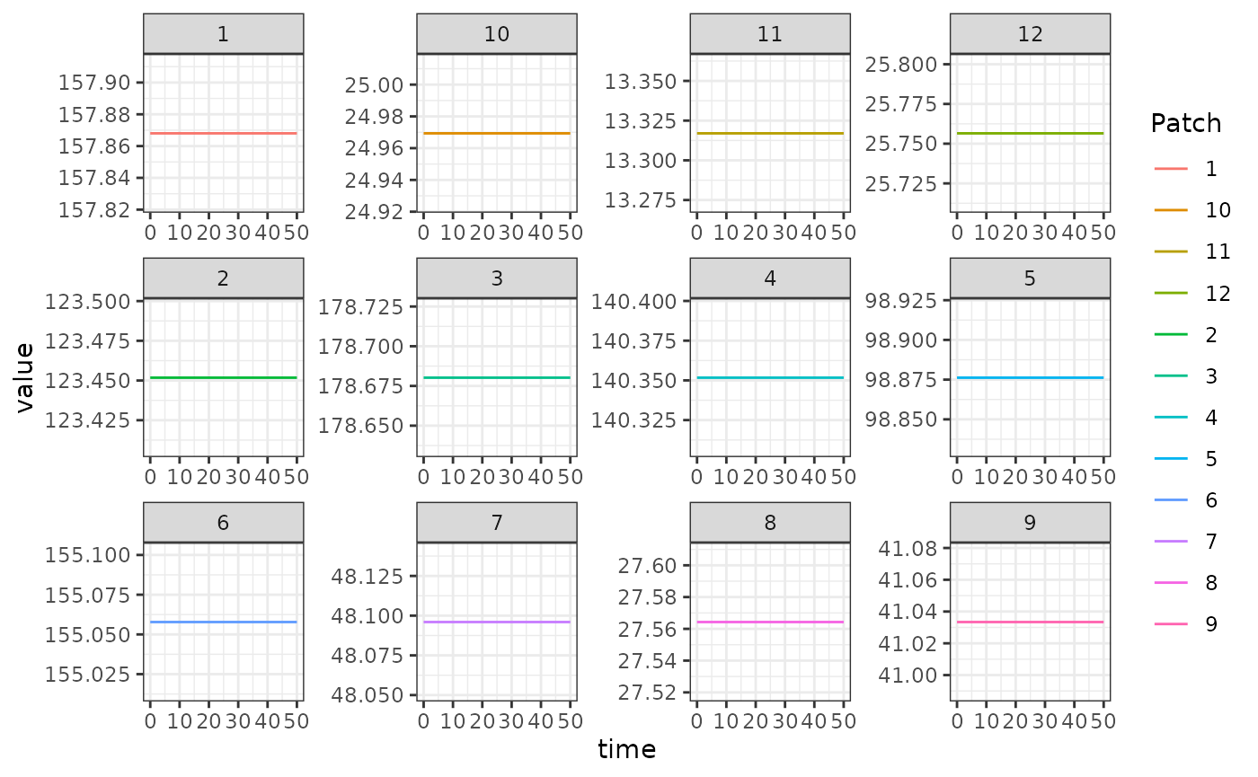
#| fig.alt: >
#|   Plottin orbits for the variables
Setup Utilities
In the vignette above, we set up a function to solve the differential
equation. We hope this helps the end user to understand how
ramp.xds works under the hood, but the point of
ramp.xds is to lower the costs of building, analyzing, and
using models. The functionality in ramp.xds can handle this
case – we can set up and solve the same model using built-in setup
utilities. Learning to use these utilities makes it very easy to set up
other models without having to learn some internals.
To set up a model with the parameters above, we make three list with the named parameters and their values. We also attach to the list the initial values we want to use, if applicable. For the Ross-Macdonald adult mosquito model, we attach the parameter values:
Each one of the dynamical components has a configurable
trivial algorithm that computes no derivatives, but passes its
output as a parameter (see human-trivial.R. To configure
Xpar, we attach the values of kappa to a
list:
Similarly, we configure the trivial algorithm for aquatic
mosquitoes (see aquatic-trivial.R).
To set up the model, we call xds_setup with
nPatchesis set to 3MYnameis set to “macdonald” to run the Ross-Macdonald model for adult mosquitoes; to pass our options, we writeMYoptions = MYo; and finally, the dispersal matrixK_matrixis passed asK_matrix=K_matrixXnameis set to “trivial” to run the trivial module for human infection dynamicsLnameis set to “trivial” to run the trivial module aquatic mosquitoes
Otherwise, setup takes care of all the internals:
xds_setup(MYname = "macdonald", Xname = "trivial", Lname = "trivial",
    nPatches=3, Koptions=K_matrix, membership = c(1:3),
    residence = c(1:3), HPop = HPop,
    MYoptions = MYo, XHoptions = Xo, Loptions = Lo) -> MYeg
Now, we can solve the equations using xds_solve and
compare the output to what we got above. If they are identical, the two
objects should be identical, so can simply add the absolute value of
their differences: