Trace Functions

library(ramp.xds)
library(viridisLite)

As part of the plug-and-play modular design for ramp.xds, each dynamical component includes a trivial model that has no variables. The outputs required by other components are passed as a trace function. These trace functions have three parts:

• a mean value, or a scaling argument

• a function that returns a F_seasonal signal, configured with a line in the appropriate options list, F_season = function(t){...}

• a function that returns a F_trend, configured with a line in the appropriate options list, F_trend = function(t){...}

Trivial Modules

The trivial modules each returns different values:

• The trivial L-component module is set up by create_Lpar_trivial. The function F_emerge() returns Lambda*F_season(t)*F_trend(t). To override the defaults, Lopts must be a named list that sets the values of the elements:

  • Lambda = c(...) is the

  • F_season = function(t){...}

  • F_trend = function(t){...}

• The trivial MYZ-component module is setup by make_MYZpar_trivial. The values will return either F_fqZ or F_eggs

  • Both F_fqZ and F_eggs use the same seasonality and trend functions:

    • F_season = function(t){...}

    • F_trend = function(t){...}

  • the function F_fqZ() returns f*q*Z*F_season(t)*F_trend(t). To configure, MYZopts should be a named list that sets the values of the elements:

    • f = c(...)

    • q = c(...)

    • Z = c(...)

  • the function F_eggs() returns eggs*F_season(t)*F_trend(t); to override the defaults, MYZopts must be a named list that sets the values of the elements:

    • eggs = c(...)

• The trivial X-component module for human / host infection and immunity is set up by create_Xpar_trivial. F_X calls F_H and then returns H*kappa*F_season(t)*F_trend(t)

  • F_H is configured in xds_setup by passing HPop = ...

  • To configure F_X, Xopts must be a named list that sets the values of the elements. The values of F_X should be in the interval $[0,H]:$

    • kappa = c(...)

    • F_season = function(t){...}

    • F_trend = function(t){...}

make_function

To make it easy to conduct thought experiments, ramp.xds has developed a system for setting up functions:

• make_function(opts) as a tool for generating functions with the right properties.

• makepar_F_* is an informal function family to construct parameter / options for make_function methods.

Seasonality

A constructor for seasonality functions drawn from a generalized family involving trigonometric functions is returned by make_function.sin with the associated makepar_F_sin that returns functions of the form: $$S(t) = c\left(1 + \epsilon + \sin\left(\frac{2 \pi (t-\tau)}{365}\right)\right)^p$$

• $c$ or norm is a normalizing constant

• $\tau$ or phase sets the timing of the peak

• $\epsilon \geq 0$ or floor is a shape parameter: increasing the values of $\epsilon$ reduces the variance

• $p \geq 0$ or pw is a shape parameter.

p1 = makepar_F_sin()
S1 <- make_function(p1)

The default normalizing constant is $365$ so that if $S$ is multiplied by some other constant, $m,$ the average daily value of the function over a year is $1.$

integrate(S1, 0, 365)$val

## [1] 365

tt <- seq(0, 3*365, by=5)
plot(tt, S1(tt), type ="l", xlab = "Time (in Days)", ylab = expression(S(t)))

p2 = makepar_F_sin(phase=120)
S2 <- make_function(p2)

plot(tt, S1(tt), type ="l", xlab = "Time (in Days)", ylab = expression(S(t)))
lines(tt, S2(tt), col = "blue")

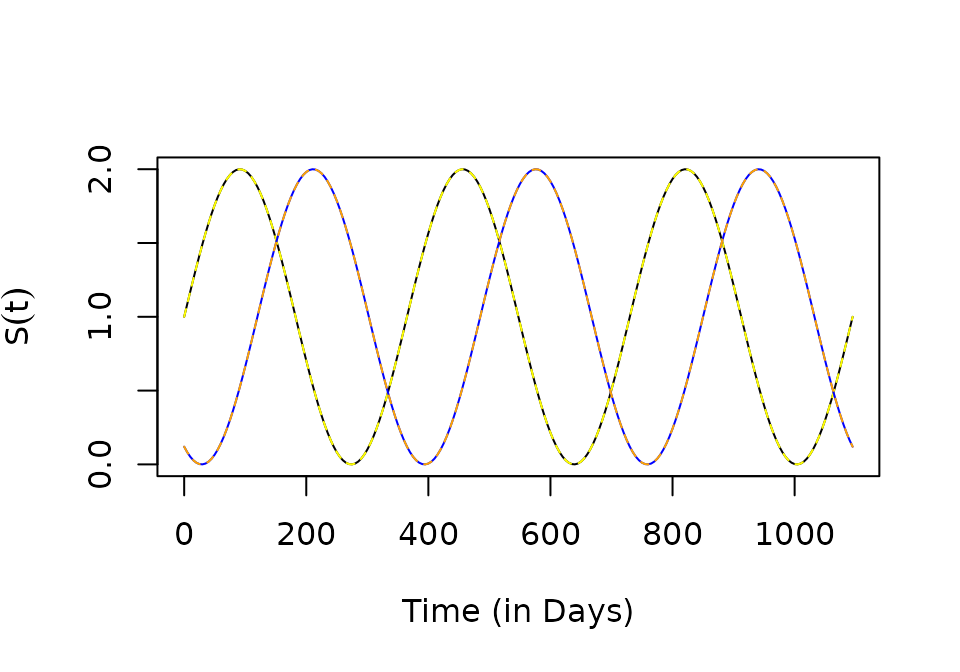
The function can return a vector of $N$ functions, each one configured as if $N=1$

p3 = makepar_F_sin(phase = c(0,120), N=2)
S3 <- make_function(p3)

s3 <- S3(tt) 
plot(tt, s3[1,], type ="l", xlab = "Time (in Days)", ylab = expression(S(t)))
lines(tt, S1(tt), col = "yellow", lty=2)
lines(tt, s3[2,], col = "blue")
lines(tt, S2(tt), col = "orange", lty=2)

p4 <- makepar_F_sin(floor=.5)
p5 <- makepar_F_sin(floor=2)
p6 <- makepar_F_sin(pw=3)
p7 <- makepar_F_sin(pw=6)

S4 <- make_function(p4)
S5 <- make_function(p5)
S6 <- make_function(p6)
S7 <- make_function(p7)

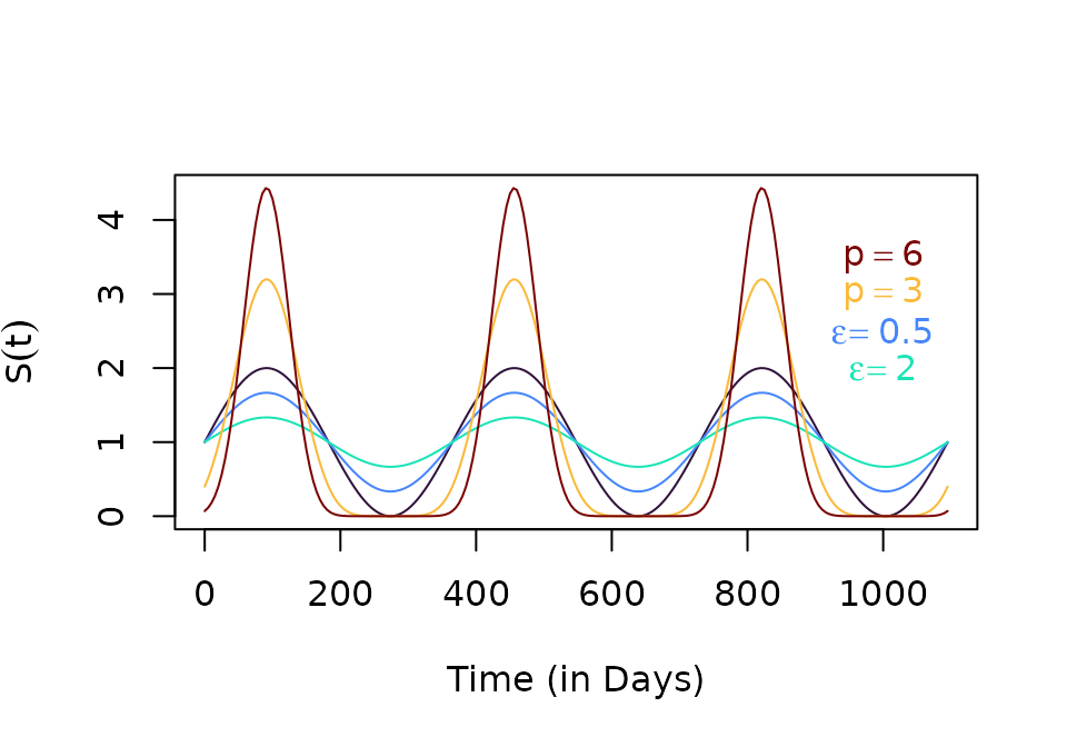
The shape parameters make it easy to configure a seasonality function with a range of features:

clrs = turbo(7)
plot(tt, S7(tt), type ="n", xlab = "Time (in Days)", ylab = expression(S(t)))
lines(tt, S1(tt), col = clrs[1])
lines(tt, S4(tt), col = clrs[2])
lines(tt, S5(tt), col = clrs[3])
lines(tt, S6(tt), col = clrs[5])
lines(tt, S7(tt), col = clrs[7])
text(1000, 3.5, expression(p==6), col=clrs[7])
text(1000, 3, expression(p==3), col=clrs[5])
text(1000, 2.5, expression(epsilon==0.5), col=clrs[2])
text(1000, 2, expression(epsilon==2), col=clrs[3])

sigmoid

ps1 <- makepar_F_sigmoid()
Fs1 <- make_function(ps1)

tt <- seq(0, 365, by=5)
plot(tt, Fs1(tt), type ="l", xlab = "Time (in Days)", ylab = expression(Fs1(t)))

sharkfin

c1 <- makepar_F_sharkfin()
C1<- make_function(c1)

tt <- seq(0, 565, by=5)
plot(tt, C1(tt), type ="l", xlab = "Time (in Days)", ylab = expression(Fs1(t)))

c2a <- makepar_F_sharkfin(L = 90, dk = 1/110)
c2b <- makepar_F_sharkfin(L = 180, dk = 1/40)

c2 <- makepar_F_sharkfin(L = c(90, 180), dk = c(1/110, 1/40), pw=c(2,1), N=2)

C2<- make_function(c2)

C2t <- C2(tt)

plot(tt, C2t[1,], type ="l", xlab = "Time (in Days)", ylab = expression(Fs1(t)))
lines(tt, C2t[2,])