The SIS Module

Xname = "SIS"

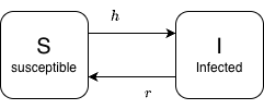
For the XH component, the SIS module implements a basic system of differential equations, that is often called the SIS compartment model (see Figure 1). This vignette describes the model and its implementation in ramp.xds. For a more mathematical introduction, see Malaria Theory – SIS Dynamics

Figure 1: A Diagram of the SIS Model

At basic setup, the SIS module with defaults is specified like this:

library(ramp.xds)
mod <- xds_setup(Xname = "SIS")

Basic Dynamics

The following describes the notation and basic setup, including variable and parameter names.

The Compartment Model

A population is subdivided into susceptible (\(S\)) and infected and infectious (\(I\)) individuals, where the total population is \(H = S+I.\)

We let \(h\) denote the force of infection (FoI).
We let \(r\) denote the clearance rate for infections.

The dynamics are described by a pair of equations:

\[ \begin{array}{rl} \frac{dS}{dt} &= -hS + rI \\ \frac{dI}{dt} &= h S - rI \end{array} \]

If \(H\) is constant, then one of these equations is redundant, and we need only compute:

\[ \frac{dI}{dt} = h (H-I) - rI \]

The model here has been implemented in the ramp.xds modular framework that handles human demography, exposure, infectiousness, and diagnostics and detection.

In the ramp.xds module, \(H\) is a variable, so we compute \(dH/dt,\) and \(dI/dt\) includes additional terms that describe demographic changes.

Exposure and \(b\)

The module handles exposure through the standard interface (see Exposure). In a nutshell:

\(E(t)\): the daily EIR is computed for each population stratum
\(b\) is a basis prameter in the SIS module describing the probability of getting infected by an infectious bite
\(h\) is the daily FoI, foi (or what Ross called the happenings rate):
- it is computed in Exposure as \(h = F_h(b, E)\)
- By default, the FoI assumes the number of bites per persion is Poisson, so the FoI is linearly proportional to the EIR: \(h = b E\)

For more, including advanced setup options, see Exposure

Infectiousness: \(c\)

Infected humans are not fully infectious. We assume that the fraction of bloodmeals on infectious humans that infect a mosquito is \(c.\) The blood feeding and transmission interface uses biting weights and availability, so we compute the infectious density of a stratum: \[F_I = c I.\]

If there is a single population stratum, then
\[\kappa = \frac {cI} H\]

Diagnostics and Detection

The probability a human would test positive is denoted \(q\), so while true prevalence is \[x=I/H,\] observed prevalence would be \[x_q=qI/H.\] The model includes three parameters for detection by light microscopy, RDT or PCR:

q_lm - the probability of detecting parasites by light microscopy
q_rdt - the probability of detecting parasites by rapid diagnostic test
q_pcr - the probability of detecting parasites by PCR

We note that in this model, the observed PR is a linear function of the true PR.

Basic Setup

During basic setup, the parameters are assigned the following default values:

b=0.55
r=1/180
c=0.15
q_lm=0.8
q_rdt=0.8
q_pcr=0.9

To inspect the parameters, use get_XH_pars. We already set up mod using the default values:

get_XH_pars(mod)$r

## [1] 0.005555556

To overwrite the defaults at setup, pass a named list to xds_setup.

mod1 <- xds_setup(Xname = "SIS", XHoptions = list(r=1/200))
get_XH_pars(mod1)$r

## [1] 0.005

To change a parameter value after setup, pass a named list to change_XH_pars.

mod <- change_XH_pars(mod, options = list(r=1/100))
get_XH_pars(mod)$r

## [1] 0.01

Mass Treatment

The module includes a port to simulate mass treatment. In the SIS model, mass treatment increases the clearance rate from \(r\) to \(r + \xi(t)\). After curing an infection, in this model, the humans become susceptible to infection again.

\[ \dot{I} = h (H-I) - \left(r+\xi\left(t\right)\right) I \]

During basic set up, the function returns no effect: \(\xi(t)=0\). Configuring a mass treatment function is handled as an advanced setup option in ramp.control (see ramp.control::Mass Treatment)

\(\xi(t)\) is either called mda(t) or msat(t): functions implementing mass treatment
- The function mda(t) implements mass drug administration
- The function msat(t) implements mass screen and treat using detection parameters (see above)
Setup for mass treatment is an advanced option in ramp.control

To read more, see ramp.control::Mass Treatment

Human Demography

The implementation of the model was generalized to consider human (or host) vital dynamics.

The population birth rate, \(B(t, H)\)
A constant per-capita rate, \(\mu.\) The model does not include a parameter to describe disease-induced mortality

\[ \frac{dH}{dt} = B(t, H) - \mu H \] These demographic changes in \(H\) require us to update the derivatives for \(S\) and \(I.\) Since newborns are susceptible, we get:

\[ \frac{dS}{dt} = B(t, H) - h S + r I - \mu S \]

The dynamics for infected individuals are:

\[ \frac{dI}{dt} = h S - r I - \mu I \] Once again, since \(H=S+I,\) one of these equations is redundant. We compute \(dH/dt\) and \(dI/dt.\)

In ramp.demog, we have implemented a generalized system called principled stratification making it possible model aging, migration, and dynamical exchanges among strata. After setup, all these dynamics are combined in a single demographic matrix \(D\). The implementation is thus more general:

\[ \dot{H} = B(t, H) - D \cdot H \]

By default, the model is implemented with static population dynamics:

\(B(t,H)\) or B(t,H) = 0: a function describing the population birth rate
\(D\) or D_matrix=0, where \(0\) is a matrix of zeros.

Other functions can be configured as advanced options in ramp.demog.

The `SIS` Module

Variables

The module has two variables:

\(H\) or H is human population density, a vector of length nStrata
- Since human population size, \(H,\) has effects on the blood feeding interface, its value must be assigned during setup as HPop=...
- The parameter nStrata is set to length(HPop)
- There is a function to change \(H\) called change_H
\(I\) or I is the density of infected humans, a vector of length nStrata
- The default initial value is \(I=1\)
- The function to change the initial values of \(I\) are called by change_XH_inits

The Derivatives

The derivatives computed by dXHdt.SIS are equivalent to:

\[ \begin{array}{rl} \dot{H} &= B(t, H) - D \cdot H \\ \dot{I} &= h (H-I) - \left(r+\xi\left(t\right)\right) I - D \cdot I \end{array} \]

Example

Here we run a simple example with 3 population strata at equilibrium. We use ramp.xds::setup_XH to set up parameters, and ramp.xds::setup_XH_inits to set the initial values. We configure a trace function to force the EIR.

Users interested in more technical details should read our fully worked multi-patch example.

First, we define the size of three population strata:

H <- c(100, 500, 250)
nStrata <- length(H)

We use the use the default model of human demography with no births or deaths.

Next, we define the parameter values for all three strata as a named list:

b <- rep(0.55, nStrata) 
c <- rep(0.15, nStrata) 
r <- rep(1/200, nStrata)

To use these values to build our model, we create a named list:

Xo = list(b=b, c=c, r=r)

We want to set up the model in a way that tests the software. We want to set values of the EIR and, knowing what the answer should be, show that we get them back. First, we set the values of the FoI, and then we compute the EIR:

foi = c(1:3)/365 
eir <- foi/b

The equilibrium values we should get back after running the equations to steady state are \(I = H h /(h+r)\)

I_eq = H*foi/(foi+r) 
I_eq

## [1]  35.39823 261.43791 155.44041

First, we use xds_setup and next, we do it the long way

Using Setup

To set up the model, we simply do this:

xds_setup_eir(eir, Xname="SIS", HPop=H, XHoptions = Xo) -> test_SIS

To solve it, we do this:

xds_solve(test_SIS)-> test_SIS

We plot the prevalence over time:

clrs = viridisLite::turbo(5)[c(1,2,5)]
xds_plot_PR(test_SIS, clr=clrs)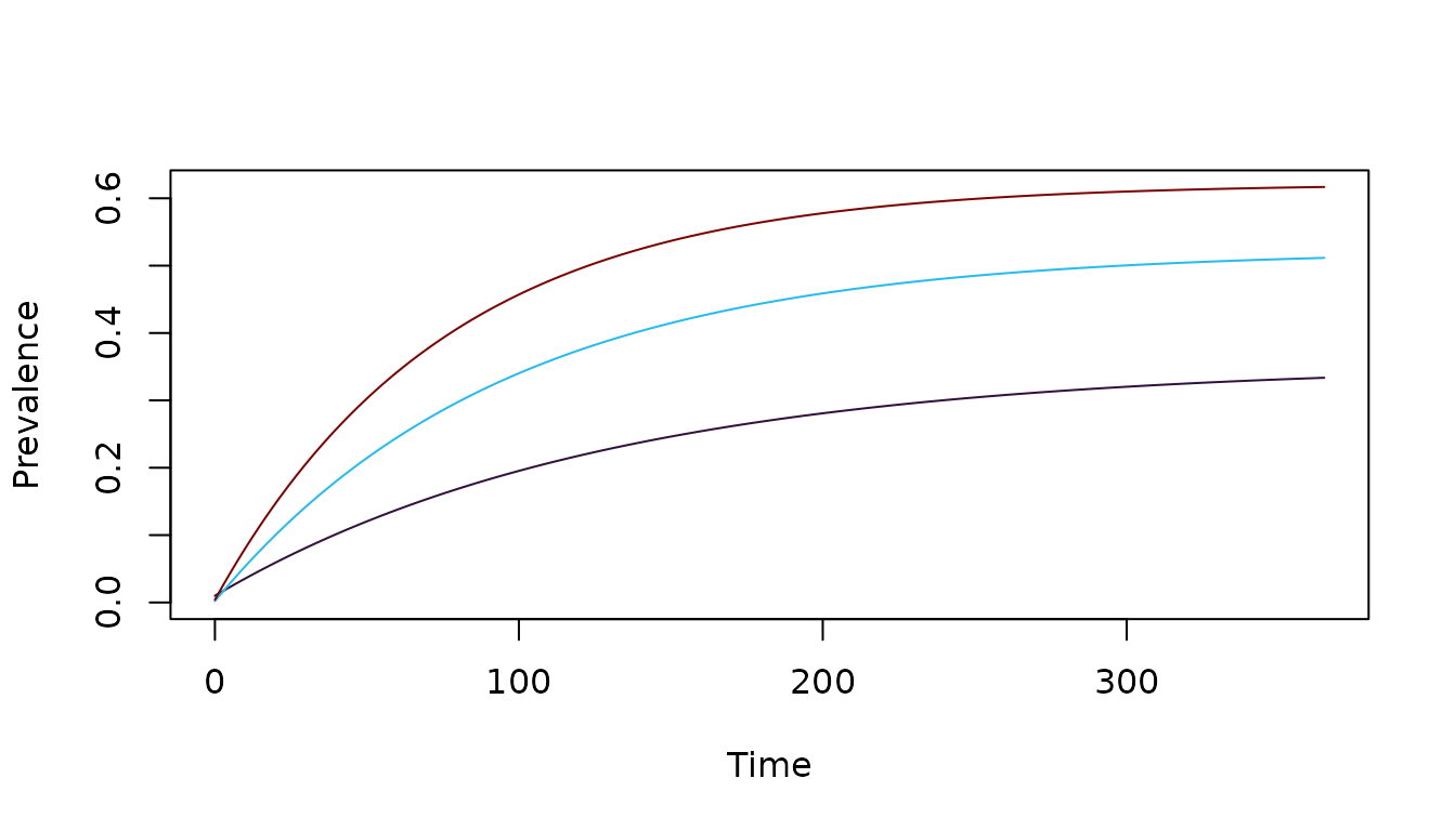

If we set the initial values of \(I\) to the steady state values, the variables shouldn’t change at all. To change the values, we simply add them to the list

test_SIS <- change_XH_inits(test_SIS, options = list(I=I_eq))
xds_solve(test_SIS)-> test_SIS 
xds_plot_PR(test_SIS, clr=clrs)

Or we can use the get_XH_out function to get the values of the orbits. This gets the return values and pulls of the the values of \(I\) at the last time step:

get_XH_out(test_SIS, 1) -> XH2
I_last <- tail(XH2$I, 1)
I_last

##               4        5        6
## [366,] 35.39823 261.4379 155.4404

sum(tail(XH2$I, 1) - I_eq)

## [1] 0

Another Test

If we set \(I(0) = 0\), the simple model has a closed form solution:

\[ I(t) = H (1-e^{-(h+r) t}) \frac{h}{h+r} \] We can reset the initial conditions and solve the system of differential equations:

test_SIS <- change_XH_inits(test_SIS, options = list(I=rep(0,3)))
xds_solve(test_SIS)-> test_SIS 
Itest = get_XH_out(test_SIS, 1)$I 
xds_plot_PR(test_SIS, clr=clrs)

…and we can compute the exact solutions for the same values of \(t\):

t = get_XH_out(test_SIS, 1)$time
It = matrix(0, 366, 3)
ss = H*foi/(r+foi)
for(i in 1:3){
  It[,i] = H[i]*(1-exp(-(r[i]+foi[i])*t))*foi[i]/(foi[i]+r[i])
}

The summing over all the squared differences is less than \(10^{-6}.\)

sum((It-Itest)^2) < 1e-6

## [1] TRUE

Generalized, Modular SIS Infection Dynamics