5-3-4 Example

library(ramp.xds)
library(expm)
library(data.table)
library(ggplot2)
library(deSolve)

Introduction

This vignette illustrates how to setup, solve, and analyze models of mosquito-borne pathogen transmission dynamics and control using modular software. It serves several purposes:

Modular notation is illustrated by constructing a model with five aquatic habitats ( $n_q=5$ ), three patches ( $n_p=3$ ), and four human population strata ( $n_h=4$ ). We call it 5-3-4.

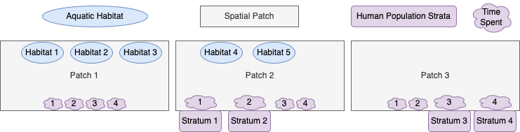
Diagram

The model 5-3-4 is designed to illustrate some important features of the framework and notation. We assume that:

the first three habitats are found in patch 1; the last two are in patch 2; patch 3 has no habitats.
patch 1 has no residents; patches 2 and 3 are occupied, each with two different population strata;
Transmission among patches is modeled using the concept of time spent, which is similar to the visitation rates that have been used in other models. While the strata have a residency (i.e; a patch they spend most of their time in), each stratum allocates their time across all the habitats.

Encoding Structural Information

Basic location information can be encoded in vectors. One vector, called the habitat membership vector or membership, holds information about the location of habitats. Another vector, called
the strata residency vector or residence, encodes the information about where people live.

For the aquatic habitats, the habitat membership vector is an ordered list of the index of patches where the habitats are found:

membership = c(1,1,1,2,2)
membership
#> [1] 1 1 1 2 2

The number of habitats, $n_q$ or nHabitats, is the length of the membership matrix:

nHabitats = length(membership)
nHabitats
#> [1] 5

For the human population strata, the residence vector is an ordered list of the index of patches where people live:

residence = c(2,2,3,3)
residence
#> [1] 2 2 3 3

The number of strata, $n_h$ or nStrata, is the length of the residence matrix:

nStrata = length(residence)
nStrata
#> [1] 4

The number of patches, $n_p$ or nPatches, is just a number:

nPatches = 3

Aquatic Habitat Membership Matrix

For computation, ramp.xds uses an $n_p \times n_q$ matrix called $\cal{N}.$ It is specified by the habitat vector. In the matrix, ${\cal N}_{i,j}$ is $1$ if the $i^{th}$ patch contains the $j^{th}$ habitat:

$$\begin{equation} {\cal N} = \left[ \begin{array}{ccccc} 1 & 1 & 1 & 0 & 0 \\ 0 & 0 & 0 & 1 & 1\\ 0 & 0 & 0 & 0 & 0\\ \end{array} \right] \end{equation}$$

The matrix is created by a function create_habitat_matrix:

habitat_matrix = create_habitat_matrix(nPatches, membership)
habitat_matrix
#>      [,1] [,2] [,3] [,4] [,5]
#> [1,]    1    1    1    0    0
#> [2,]    0    0    0    1    1
#> [3,]    0    0    0    0    0

The habitat matrix is used to sum quantities in habitats up to patches. For example, the number of habitats per patch is ${\cal N} \cdot 1$, where $1$ is a vector of 1’s:

as.vector(habitat_matrix %*% rep(1,5)) 
#> [1] 3 2 0

The Residence Matrix

For computation, ramp.xds also creates a $n_p \times n_h$ matrix called $\cal J.$ It is specified by residence vector. The element ${\cal J}_{i,j}$ is $1$ if the $j^{th}$ stratum resides in the $i^{th}$ patch:

$$\begin{equation} {\cal J} = \left[ \begin{array}{cccc} 0 & 0 & 0 & 0 \\ 1 & 1 & 0 & 0 \\ 0 & 0 & 1 & 1 \\ \end{array} \right] \end{equation}$$

The matrix is created by a function create_residence_matrix:

residence_matrix = create_residence_matrix(nPatches, residence)
residence_matrix
#>      [,1] [,2] [,3] [,4]
#> [1,]    0    0    0    0
#> [2,]    1    1    0    0
#> [3,]    0    0    1    1

The number of strata per patch is:

as.vector(residence_matrix %*% rep(1,4)) 
#> [1] 0 2 2

Egg Laying

It is plausible that these habitats are not all found with the same propensity. Habitats are found after a search, and that search begins after mosquitoes have blood fed. To compute egg distribution, we create a vector describing habitat search weights, denoted $\omega.$ The proportion of eggs laid in each patch is it’s search weight as a proportion of summed search weights of all habitats in a patch, a quantity that we have called availability, $Q$ .

For now, we generate arbitary weights for each one of the habitats:

searchWtsQ = c(7,2,1,8,2)
searchWtsQ
#> [1] 7 2 1 8 2

And we can compute availability as $\cal N \cdot w$. In ramp.xds, the function that computes habitat availability is called compute_Q:

Q <- compute_Q(habitat_matrix, searchWtsQ)
Q
#> [1] 10 10  0

Eggs are distributed among habitats in proportion to the relative values of the habitat search weights. These habitat search weights and availability can be used to compute the values of some adult mosquito bionomic parameters using functional responses, that make use of their absolute values. The absolute values only have a meaning through their effects.

The egg dispersal matrix $\mathcal{U}$ is a $n_q \times n_p$ matrix describing how eggs laid by adult mosquitoes in a patch are allocated among the aquatic habitats in that patch. It is a matrix of search weights normalized by availability:

$$\begin{equation} {\cal U} = \left[ \begin{array}{ccccc} .7 & 0 & 0\\ .2 & 0 & 0\\ .1 & 0 & 0\\ 0 & .8 & 0\\ 0 & .2 & 0\\ \end{array} \right] \end{equation}$$

It is computed using the function compute_calU that takes care of a problem that could arise from having empty patches, like patch 3 in this model.

calU = compute_calU(searchWtsQ, habitat_matrix, Q)
calU
#>      [,1] [,2] [,3]
#> [1,]  0.7  0.0    0
#> [2,]  0.2  0.0    0
#> [3,]  0.1  0.0    0
#> [4,]  0.0  0.8    0
#> [5,]  0.0  0.2    0

Blood Feeding

Blood feeding is an activity that involves mosquitoes and humans: mosquitoes are searching for vertebrate hosts to feed on, and they find and feed on humans and other vertebrate hosts. The blood feeding constructs in ramp.xds translate this into a set of algorithms. The host population can be subdivided into a set of strata, and those humans spend time in the patches around home. Both humans and mosquitoes have daily activity patterns, so that human time spent and relative mosquito activity rates can change during the day. Time spent is thus translated into time at risk. Like the habitats, the availability of those hosts to blood feeding mosquitoes is affected by a set of search weights.

This model has four population strata with even search weights:

searchWtsH = c(1,1,1,1)

This size of each population stratum differs:

HPop <- c(10,90, 100, 900)

The time spent matrix, $\Theta$ is a $n_p \times n_h$ matrix. Each column describes how a human stratum allocates time among patches.

$\begin{equation} \Theta = \left[ \begin{array}{cccc} 0.01 & .01 & .001 & .001 \\ 0.95 & .92 & .04 & .02 \\ 0.04 & .02 & .959 & .929 \\ \end{array} \right] \end{equation}$

This model does not consider daily patterns in human or mosquito activity, so time spent and time at risk are identical.

TaR <- t(matrix(
 c(c(0.01,0.01,0.001,0.001),
  c(.95,.92,.04,.02),
  c(.04,.02,.959,.929)), 4, 3
))

The availability of hosts is of time at risk and the population density weighed by their search weights:

W <- compute_W(searchWtsH, HPop, TaR)
W
#> [1]   2.0 114.3 934.2

Transmission

A mixing matrix, $\beta$ , describes the expected proportion of each infective bite that would be received be each population stratum.

compute_beta(HPop, W, searchWtsH, TaR)
#>       [,1]         [,2]         [,3]
#> [1,] 5e-03 0.0083114611 4.281738e-05
#> [2,] 5e-03 0.0080489939 2.140869e-05
#> [3,] 5e-04 0.0003499563 1.026547e-03
#> [4,] 5e-04 0.0001749781 9.944337e-04

Aquatic Mosquito Dynamics

For this simulation, we use the basic competition model of larval dynamics called basicL (see more here). It requires specification of three parameters, $\psi$ (maturation rates), $\phi$ (density-independent mortality rates), and $\theta$ (density-dependent mortality terms), and initial conditions. The function ramp.xds::xde_make_Lpar_basicL does basic checking of the input parameters and returns a list with the correct class for method dispatch. The returned list is attached to the main parameter list with name Lpar.

psi <- rep(1/8, nHabitats)
phi <- rep(1/8, nHabitats)
theta <- c(1/10, 1/20, 1/40, 1/100, 1/10) 

Lpar = create_Lpar_basicL(nHabitats, psi=psi, phi=phi, theta = theta)

Adult Mosquito Dynamics

It also uses the Ross-Macdonald model (see more here). Part of the specification of parameters includes the construction of the mosquito dispersal matrix $\mathcal{K}$ , and the mosquito demography matrix $\Omega$ . Like for the aquatic parameters, we use ramp.xds::make_parameters_MYZ_RM_ode to check parameter types and return a list with the correct class for method dispatch.

The parameter values are:

g <- 1/12 
sigma <- 1/12/2 
mu <- 0 
f <- 1/3 
q <- 0.9 
nu <- c(1/3,1/3,0)  
eip <- 12 
eggsPerBatch <- 30

We create a named list:

MYZo = list(g=g, sigma=sigma, mu=mu, f=f, q=q, nu=nu, eip=eip, eggsPerBatch=eggsPerBatch)

Mosquito dispersal among the patches is described by a matrix, $\cal K.$ Each column in $\cal K$ describes the proportion of emigrating mosquitoes that go to every other patch. The diagonal elements are all $0$ :

calK <- t(matrix(
 c(c(0, .6, .3), 
  c(.4, 0, .7), 
  c(.6, .4, 0)), 3, 3))

We construct the demographic matrix $\Omega$ given by the formula $$\Omega = \mbox{diag}\left(g\right) - \left[\mbox{diag}\left(1-\mu\right) - {\cal K} \right] \cdot \mbox{diag}\left(\sigma\right)$$ It is computed by compute_Omega_xde:

Omega <- compute_Omega_xde(g, sigma, mu, calK)

Survival and dispersal through the EIP in this model, denoted $\Upsilon,$ is computed using matrix exponentiation:

Upsilon <- expm::expm(-Omega*eip)

The function xde_make_MYZpar_RM can be used to construct the adult mosquito model object, called MYZpar.

MYZpar = create_MYZpar_macdonald(nPatches, MYZo) 
class(MYZpar) <- "macdonald"

The parameters are assigned to a list called baseline so that it can be stored and used to compute the values of bionomic parameters that have been modified by control.

names(MYZpar)
#>  [1] "nPatches"     "eip"          "f"            "q"            "g"           
#>  [6] "sigma"        "mu"           "nu"           "eggsPerBatch" "calK"        
#> [11] "Omega"        "Upsilon"      "baseline"

Human Infection Dynamics

We use a static demographic model, which assumes a constant population size (constant $H$ ).

The 5-3-4 model uses the basic SIS (Susceptible-Infected-Susceptible) model for the human component (see more here). It can be configured using ramp.xds::xde_make_Xpar_SIS.

r <- 1/200
b <- 0.55
c <- c(0.1, .02, .1, .02)

The model is configured and assigned the name Xpar:

Xpar <- create_Xpar_SIS(nStrata, list(), b, r, c)

Initial Conditions

To solve the model, each variable needs an initial value. For the aquatic model:

Linits <- list(
  L = rep(1, nHabitats)
)

For the adult mosquito model:

MYZinits = list(
  M = rep(100, nPatches),
  P = rep(10, nPatches),
  Y = rep(1, nPatches),
  Z = rep(0, nPatches)
)

For the human model:

Xinits = list(I = as.vector(0.2*HPop))

The `xds` Template

To build a model, ramp.xds must create an template that stores the information about the patches, habitats, and strata in a rigid form. The functions that solve and analyze the systems of differential equations are, like most computer programs, unforgiving. An object describing a model that can be solved by ramp.xds is called an xds object. ramp.xds supports nimble model building for extensible dynamical systems, including extensible systems of differential equations (xde), and discrete-time systems using difference equations (dts).

Since the software is designed to solve very complex systems, we will need to create an object that could accommodate added realism (e.g. vector control). The function make_xds_template sets up a compound list in R that is like a building that we anticipate modifying, with ports and junctions ready. These capabilities that are not needed by simple models. The software’s requires that some objects are present to handle all that complexity. Since most users won’t want to learn about the details, the software includes a function, called make_xds_template that sets up the scaffolding for a model, including many that are set to their null values (turned off).

A user only needs to know how to encode the information and what information to encode. The rest is handled by functions. It is helpful for users to understand some of the notation and terms. The following are set up in order by make_xds_template:

the first required argument sets the value and class of xds
- xde is for extensible systems of differential equations
- dts is for not a discrete-time systems
the second required arugment sets the value and class of frame that dispatches both a setup function and a class of xde_derivatives (for xde models) or a class of dts_update (for dts models)
- full tells us the model should configure and compute all three dynamical components
- Other options – mosy, aquatic, human, and cohort – work on subsets of the components, and while they could be configured using full
the third required term sets the value ofdlay that dispatches xds_solve
- ode uses deSolve::ode for ordinary differential equations,
- dde uses deSolve:dde for delay differential equations
the next three arguments are nPatches and membership and residence, as explained above.

params = make_xds_template("dde", "full", nPatches, membership, residence)

After being set up:

c(params$nHabitats, params$nPatches, params$nStrata)
#> [1] 5 3 4

This was created by make_xds_template and stored as params$habitat_matrix

params$habitat_matrix
#>      [,1] [,2] [,3] [,4] [,5]
#> [1,]    1    1    1    0    0
#> [2,]    0    0    0    1    1
#> [3,]    0    0    0    0    0

If we want to retrieve the membership matrix, we can call view_habitat_matrix

view_habitat_matrix(params)
#> $habitat_index
#> [1] 1 2 3 4 5
#> 
#> $patch_membership
#> [1] 1 1 1 2 2

The function make_xds_template was designed to create a scaffolding. So Q and calU get created with default values: Iall patches are assumed to have the same biting weights.

params$vars$Q
#> [[1]]
#> [1] 3 2 0

A little detail to note is that an xds object is designed to handle multiple vector and multiple host species. The function make_xds_template only sets up the first species. Similarly, we can view the egg distribution matrix for the first species:

params$calU[[1]]
#>           [,1] [,2] [,3]
#> [1,] 0.3333333  0.0    0
#> [2,] 0.3333333  0.0    0
#> [3,] 0.3333333  0.0    0
#> [4,] 0.0000000  0.5    0
#> [5,] 0.0000000  0.5    0

While this is a reasonable way to start, we don’t want to get stuck using the default values.

To make a modular system that works as expected, we need to adopt some conventions for setting the values of parameters. This can create challenges because after changing the search weights, we will also need to update habitat availability and the egg distribution matrix. Updating all of that by hand would be cumbersome, so ramp.xds has adopted some conventions for changing parameter values and then updating the objects that depend on them.

Building the Object

params$Lpar = list() 
params$Lpar[[1]] = Lpar 
params$MYZpar = list() 
params$MYZpar[[1]] = MYZpar 
params$Xpar = list() 
params$Xpar[[1]] = Xpar

params <- make_Linits(params, 1, Linits)
params <- make_MYZinits(params, 1, MYZinits)
params <- make_Xinits(params, HPop, 1, Xinits)

params <- setup_Hpar_static(params, 1)

After the parameters for 5-3-4 have been specified, we can generate the indices for the model and attach them to the parameter list.

params = make_indices(params)

Setting Parameter Values

To assign new values for the habitat search weights, we use a function called set_habitat_wts_static. After setting the values of the habitat search weights, we need to update habitat availability and the egg distribution matrix. The functions makeQ and make_calU do this.

params <- change_habitat_weights(params, searchWtsQ)
params <- make_Q(params)
params <- make_calU(params)

We can check to see

params$vars$Q[[1]]
#> [1] 10 10  0

params$calU[[1]]
#>      [,1] [,2] [,3]
#> [1,]  0.7  0.0    0
#> [2,]  0.2  0.0    0
#> [3,]  0.1  0.0    0
#> [4,]  0.0  0.8    0
#> [5,]  0.0  0.2    0

params <- change_TimeSpent(TaR, params)
params <- make_TaR(params)

params$TimeSpent
#> [[1]]
#>      [,1] [,2]  [,3]  [,4]
#> [1,] 0.01 0.01 0.001 0.001
#> [2,] 0.95 0.92 0.040 0.020
#> [3,] 0.04 0.02 0.959 0.929

params$TaR
#> [[1]]
#> [[1]][[1]]
#>      [,1] [,2]  [,3]  [,4]
#> [1,] 0.01 0.01 0.001 0.001
#> [2,] 0.95 0.92 0.040 0.020
#> [3,] 0.04 0.02 0.959 0.929

params <- change_blood_weights(params, searchWtsH)
y0 <- get_inits(params)
params <- make_WB(0, params, y0)

params$vars$W[[1]]
#> [1]   2.0 114.3 934.2

params <- change_calK(calK, params)
params$MYZpar[[1]]$calK
#>      [,1] [,2] [,3]
#> [1,]  0.0  0.6  0.3
#> [2,]  0.4  0.0  0.7
#> [3,]  0.6  0.4  0.0

get_Omega(params, 1) 
#>             [,1]        [,2]        [,3]
#> [1,]  0.12500000 -0.02500000 -0.01250000
#> [2,] -0.01666667  0.12500000 -0.02916667
#> [3,] -0.02500000 -0.01666667  0.12500000

get_Upsilon(params, 1) 
#>            [,1]       [,2]       [,3]
#> [1,] 0.23643097 0.07241259 0.04640076
#> [2,] 0.05790317 0.23926276 0.08391499
#> [3,] 0.07354531 0.05620409 0.23756369

Functions like set_habitat_wts_static are designed to modify parameters to guarantee that all the internal objects that rely on those parameters get updated. If we use set_habitat_wts_static the updating gets done automatically.

The software was designed to handled more complex situations than the one we’ve illustrated here. In some models, we might want to make the habitat search weights change dynamically. For example, we might want to simulate habitat dynamics with some ephemeral habitats that dry up and can’t be found. That would be called a non-autonomous system, and we would need to recompute the $Q$ and $\cal U$ each time step. The egg laying object is assigned a class dynamic for dispatching by R’s S3 object system. If none of the values affecting egg laying are time dependent – we would call the resulting system autonomous – then we assign the objects a class static so they don’t get updated. To guarantee that we are recomputing things correctly, whenever the software updates the values of static parameters, it assigns the class setup. Whenever EggLaying.setup gets called, it runs EggLaying.dynamic once and then changes the class to static.

Solving

Now we can get the initial conditions of the model.

params <- make_indices(params)

Numerical Solution

Now we can pass the vector of initial conditions, y, our parameter list params, and the function ramp.xds::xde_derivatives to the differential equation solvers in deSolve::ode to generate a numerical trajectory. The classes of Xpar, MYZpar, and Lpar in params will ensure that the right methods are invoked (dispatched) to solve your model.

We need to get the stored initial values, but by default these are returned as a named list, to make it easy to examine.

y0 <- get_inits(params)
names(y0)
#> [1] "L"   "MYZ" "X"

We want to pass an unnamed vector to the solver so:

y0 = get_inits(params, flatten=TRUE)

out <- deSolve::dede(y = y0, times = seq(0, 735, by =15),
                    func = xde_derivatives, parms = params)
out1 <- out

Plot Output

With a small amount of data wrangling made easier by the data.table package, we can plot the output.

colnames(out)[params$ix$L[[1]]$L_ix+1] <- paste0('L_', 1:params$nHabitats)
colnames(out)[params$ix$MYZ[[1]]$M_ix+1] <- paste0('M_', 1:params$nPatches)
colnames(out)[params$ix$MYZ[[1]]$P_ix+1] <- paste0('P_', 1:params$nPatches)
colnames(out)[params$ix$MYZ[[1]]$Y_ix+1] <- paste0('Y_', 1:params$nPatches)
colnames(out)[params$ix$MYZ[[1]]$Z_ix+1] <- paste0('Z_', 1:params$nPatches)
colnames(out)[params$ix$X[[1]]$X_ix+1] <- paste0('X_', 1:params$nStrata)

out <- as.data.table(out)
out <- melt(out, id.vars = 'time')
out[, c("Component", "Stratification") := tstrsplit(variable, '_', fixed = TRUE)]
out[, variable := NULL]

ggplot(data = out, mapping = aes(x = time, y = value, color = Stratification)) +
 geom_line() +
 facet_wrap(. ~ Component, scales = 'free') +
 theme_bw()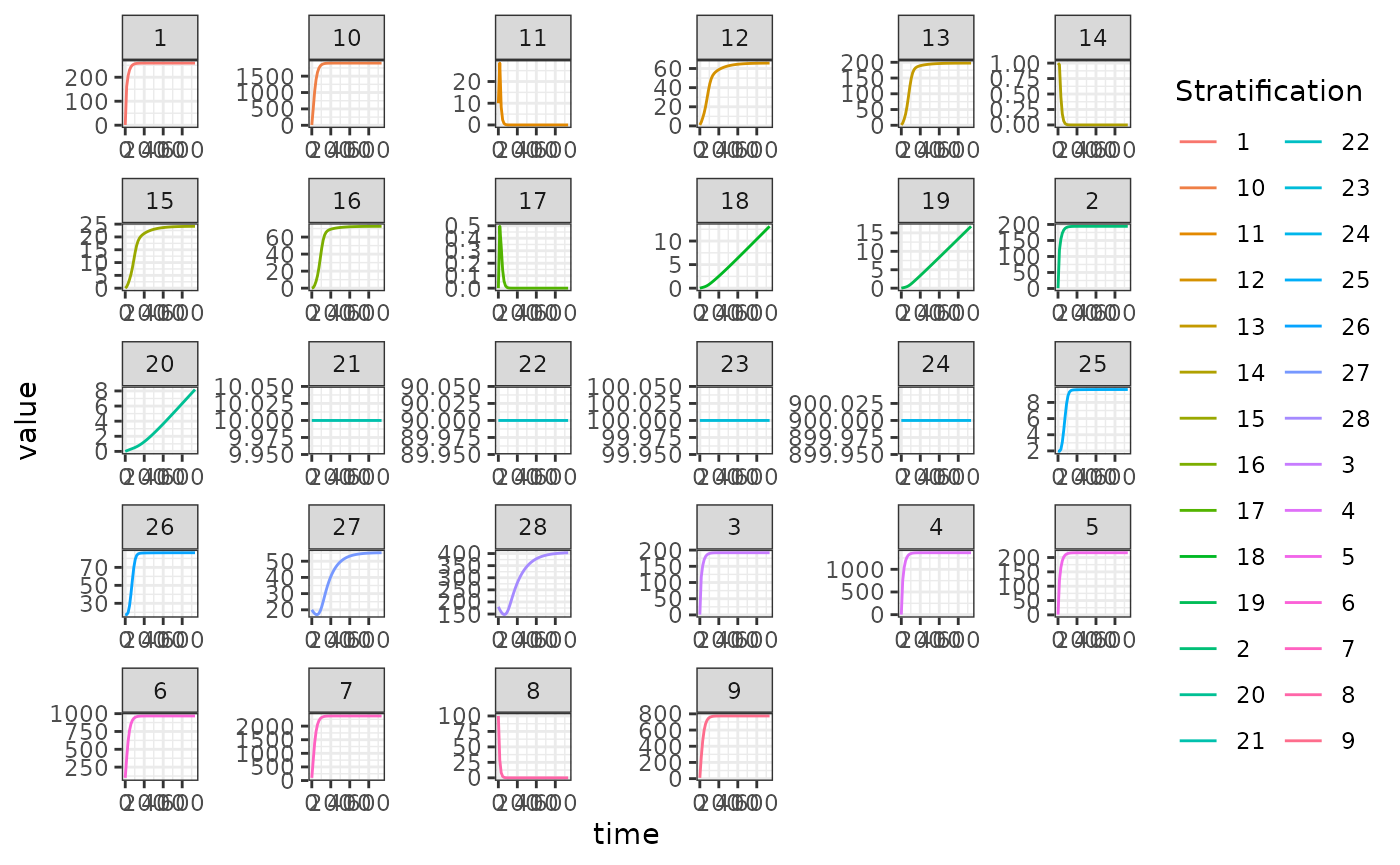

Using `xde_setup`

We create lists with all our parameters values:

MYZo = list(
 g = 1/12, sigma = 1/12/2,
 f = 1/3, q=0.9, nu=c(1/3,1/3,0),
 eggsPerBatch = 30, 
 eip = 12, 
 M = 100,  P = 10,  Y = 1, Z = 0 
)

Lo = list(
 L = 1,  
 psi = 1/8, phi = 1/8, 
 theta = c(1/10, 1/20, 1/40, 1/100, 1/10) 
)

Xo = list(
 I = as.vector(0.2*HPop),
 r = 1/200,
 b = 0.55,
 c = c(0.1, .02, .1, .02)
)

xds_setup(MYZname="macdonald", Xname="SIS", Lname="basicL", 
  nPatches = 3, HPop=c(10, 90, 100, 900), 
  membership=c(1,1,1,2,2), 
  MYZopts=MYZo, calK=calK, Xopts=Xo, Lopts = Lo,
  residence=c(2,2,3,3), searchB=searchWtsH, 
  TimeSpent=TaR, searchQ = c(7,2,1,8,2)) -> mod534

We solve and take the differences to check:

mod534 <- xds_solve(mod534, Tmax=735, dt=15)
mod534$outputs$orbits$deout -> out2

xds_plot_M(mod534, llty = c(1:3))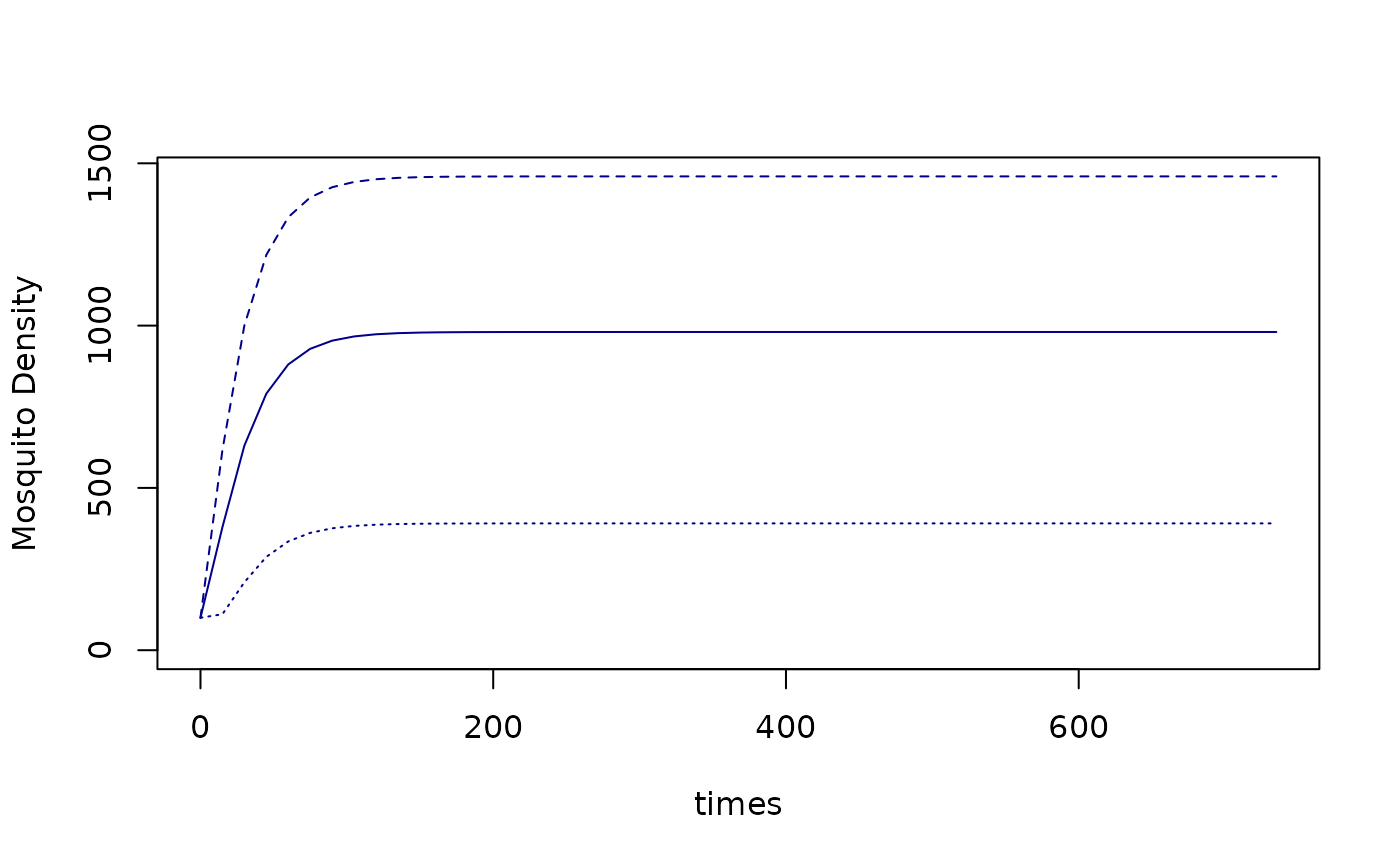

Interestingly, the differences are small:

sum((tail(out2,1) - tail(out1, 1))^2)
#> [1] 0

approx_equal(tail(out2, 1), tail(out1,1), tol = 1e-5)
#> logical(0)