This vignette gives a basic introduction to
ramp.xds and a quick demonstration.
How to install
ramp.xds-
A demonstration:
Set up a model
Solve it
Next: Working with Models
Additional documentation is available in the SimBA Project website.
ramp.xds was developed to reduce the
costs of building, solving, analyzing, and using models describing the
epidemiology, transmission dynamics and control of malaria and other
mosquito-transmitted pathogens.
Installation
The software was developed in RStudio. To download the R package, run these commands:
Then load ramp.xds:
Additional modules and functionality are available in companion
R-packages, including ramp.library,
ramp.control,
ramp.forcing,
and ramp.demog.
For more information, see the SimBA
Project website.
Setup
ramp.xds makes it easy to build and use
models for the transmission dynamics and control of malaria or other
mosquito-borne pathogens. Model building in
ramp.xds starts with a function called
xds_setup(). All arguments in xds_setup() are
assigned default values, so calling xds_setup() with no
arguments returns a fully configured model with all the default
settings.
model <- xds_setup()The object returned by xds_setup() is called an
xds model object: it is a fully defined model that can
be solved by xds_solve(). Here, we called it
model.
The arguments are stored and can be easily retrieved. The name of the
module for human / host infection and immune dynamics is stored as
Xname. The default module is the SIS
compartmental model:
model$Xname## [1] "SIS"SIS was set up with default parameter values that can be
viewed with the function get_XH_pars:
get_XH_pars(model)## $b
## [1] 0.55
##
## $c
## [1] 0.15
##
## $r
## [1] 0.005555556
##
## $q_lm
## [1] 0.8
##
## $q_rdt
## [1] 0.8
##
## $q_pcr
## [1] 0.9Functions like get_XH_pars are designed to help users
get to know the model object. In this case, the parameters are stored as
model$XH_obj[[i]], for the \(i^{th}\) species. Knowing the names, the
parameters can then be viewed (or changed). For example, this would
change r for the first species:
model$XH_obj[[1]]$r <- 1/150To make it easy to change parameters, we also wrote the
change_XH_pars function, which takes new values in a named
list.
model <- change_XH_pars(model, 1, list(r=1/150))
get_XH_pars(model)$r
## [1] 0.006666667Similarly, initial values were assigned default values at setup. In
ramp.xds, human/host demography is treated
as a distinct process, so the initial values are:
get_XH_inits(model, 1)## $H
## [1] 1000
##
## $I
## [1] 1The default parameters and initial values can be overwritten at setup
by passing options = list(...) with different values. Since
xds_setup calls functions to set up several model objects,
each component has its own options name. For the XH
component, options are passed in XHoptions:
Xo = list(r=1/150, c=0.2, b=0.6, I=2)
model1 <- xds_setup(XHoptions = Xo)
get_XH_pars(model1)
## $b
## [1] 0.6
##
## $c
## [1] 0.2
##
## $r
## [1] 0.006666667
##
## $q_lm
## [1] 0.8
##
## $q_rdt
## [1] 0.8
##
## $q_pcr
## [1] 0.9In the SIS model, we set \(H=S+I,\) so the software computes \(dH/dt\) and \(dI/dt\) and sets \(S=H-I.\) By policy, the software computes
the total population size, \(H,\)
dynamically and treats it differently. This is because it plays an
important role in setting up the Blood Feeding interface, so it
is not possible to set \(S.\) Instead,
\(S\) is computed after solving and
parsing.
get_XH_inits(model1)## $H
## [1] 1000
##
## $I
## [1] 2To change the human population density, use the change_H
function.
model1 <- change_H(1004, model1)
get_XH_inits(model1)
## $H
## [1] 1000
##
## $I
## [1] 2The module for adult mosquito ecology and infection dynamics is
called MYname. The default module is an SI model:
model$MYname## [1] "SI"The design pattern is followed. Parameters can be viewed with
get_MY_pars. Parameter values can be set by passing a named
list to MYoptions in xds_setup(), and changed
after setup by passing new values in a named list to
change_MY_pars.
The name of the default module for aquatic mosquito ecology is called
Lname. The default module is the trivial
module:
model$Lname## [1] "trivial"For the trivial module, arguments passed at the command
line configure functions that pass values to other dynamical
components.
The design pattern is followed: parameters can be viewed with
get_L_pars and the method for setting parameter values is
to pass a named list of values to Loptions in
xds_setup(). After setup, the change_L_pars
works in the same way as the other change_ functions.
Solving
After setting up, model has an empty placeholder for
outputs:
model$outputs ## list()Calling xds_solve(model) returns solutions to the
initial value problem(s): xds_solve calls
deSolve, and the values of the dependent variables at a set
of time points are attached as model$outputs.
There are three ways to pass the argument time to
deSolve: first, xds_solve can set up a vector
of time points seq(0, Tmax, by = dt) that are configurable
with the arguments Tmax and dt; second, if no
arguments are passed for time, then it uses the defaults
Tmax=365 and dt=1; third, deSolve
will use the optional argument times if it is supplied. All
four of the following do the same thing:
model <- xds_solve(model, times=0:365)
model <- xds_solve(model, times=0:365, Tmax=730, dt=5)
model <- xds_solve(model, Tmax=365, dt=1)
model <- xds_solve(model)
Internally, these are handled by the function
make_times_xde for systems of differential equations, and
make_times_dts for discrete time systems.
Note xds_solve requires an
xds model object and that it
returns an xds model object. In
this case, the function passes model and the return value
replaces model. Before xds_solve,
model$outputs was an empty list. After solving, the outputs
are stored as model$outputs:
names(model$outputs)## [1] "deout" "time" "last_y" "orbits"The outputs from solving a system of equations include:
-
deout– the raw (unparsed) outputs
-
time– the time points where dependent variables were computed -
last_y– the last state of the system
-
orbits– solutions with the values of the dependent variables and terms parsed by name, accessible separately for each dynamical component
Note that time is the set of time points where we output
the values of the dependent variables.
head(model$outputs$time, 5)## [1] 0 1 2 3 4
tail(model$outputs$time, 3)## [1] 363 364 365When xds_solve is called, the xds
model object it returns has replaced any old values. If nothing
has changed, then the outputs will be identical.
On the other hand, if anything has changed, any old outputs will get replaced. If the outputs need to be saved for future analyses, the user will probably have to write a wrapper function that extracts and saves it.
Outputs
To make it easy to deal with the outputs, the dependent variables are
parsed and returned in named lists. xds_solve() also
computes some standard terms that are likely to be of
interest.
Functions like get_EIR() make it easy to examine or save
a set of standard outputs without delving into the details.
##              [,1]
## [1,] 0.0002850000
## [2,] 0.0002685853
## [3,] 0.0002673418
Visualization
ramp.xds includes functions to plot
standard outputs:
xds_plot_Xplots the density of infected individualsxds_plot_Mplots the density of adult female mosquitoes in each patchxds_plot_Yplots the density of infected adult female mosquitoes in each patchxds_plot_Zplots the density of infectious adult female mosquitoes in each patchxds_plot_PRplots the true prevalence of infection in the human / host populationxds_plot_EIRplots the EIR for each one of the human / host population strata
par(mfrow = c(2,2))
xds_plot_X(model)
xds_plot_M(model)
xds_plot_Y(model, add=T)
xds_plot_Z(model, add=T)
xds_plot_PR(model)
xds_plot_EIR(model)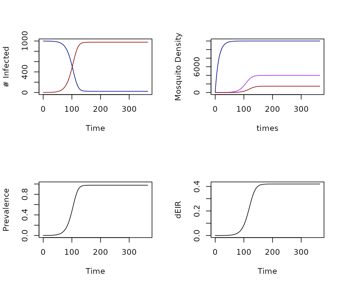
Figure 1: Plotting standard outputs
Trace
The software was designed to be fully modular, so that any module for
one dynamical component can be replaced with another. The models
included in ramp.xds illustrate its
features and ensure that the software is working as designed.
A basic requirement for full modularity is that every dynamical
component must include a trivial module. In the
trivial module, no variables are defined, but the dynamical
terms needed by related dynamical components are passed by a
configurable trace function with a generic form:
The default for the aquatic mosquito dynamical component is the
trivial module, where the mean is called
Lambda.
It is easy to change the trace function. First, we
define F_season and change the mean value of
Lambda. To set up a seasonality function, we pass a
parameter set from makepar_F_sin:
Lo = list(
       Lambda=400,
       season_par=makepar_F_sin()
      )
We use the first model as a template for the new model, but we assign
the return value a new name model_1 so that the original
one still exists:
model_1 <- setup_L_obj("trivial", model, 1, options=Lo)We want to change the initial values of model_1. Since
model_1 was copied from model, the last values
from solving it are available, and we can use a function
last_to_inits to set the initial values.
model_1 <- last_to_inits(model_1)Now, we solve to get the orbits every five days over a three-year period.
model_1 <- xds_solve(model_1, Tmax=365*3, dt=5) After solving, we can plot the orbits.
par(mfrow = c(1,2))
xds_plot_X(model_1)
xds_plot_M(model_1)
xds_plot_Y(model_1, add=T)
xds_plot_Z(model_1, add=T)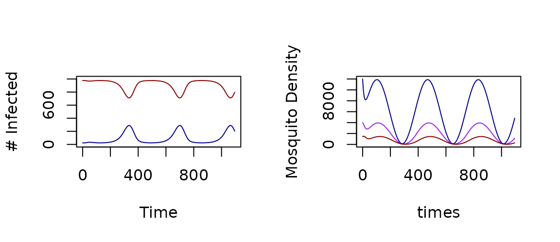
Figure 2: Outputs with Seasonal Forced Emergence using a Trace Function
Next Steps
Two good next steps are the vignettes: + Working with Models. + Basic Setup.