Modular Forms for Disease Dynamics

Introduction

Modular forms for disease dynamics are stylized ways of writing the dynamical systems that emphasize their modular structure. A mathematical framework for building models of malaria dynamics and control (and other mosquito-borne pathogens) was described in Spatial Dynamics of Malaria Transmission, and the framework was implemented in exDE. The forms we describe here rewrite models so that they closely resemble their implementation in exDE, which makes it possible to relate written equations and computed code. (Also, see the closely related vignette Understanding exDE.)

The Modular Form

We illustrate by writing a Ross-Macdonald model in its modular form (Figure 1). In its classical form, this is the model:

\[ \begin{array}{rl} dX/dt &= b e^{-gn}fq \frac YH (H-X) - r X \\ dY/dt &= a c \frac XH (M-Y) - g Y \end{array}\]

The model is explained below.

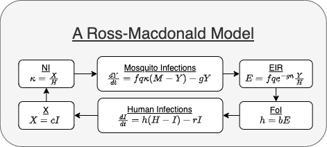
Figure 1 - Diagram of a Ross-Macdonald model as it is written in its modular form.

Parasite Infection Dynamics in Humans, $\cal X$

The equation describing human infections is written in the following way:

\[ dI/dt = h (H-I) - r I \]

where:

$I$ is the density of infected and infectious humans;
$H$ is the density of humans;
$h$ is the force of infection (FoI), the number of infections, per perspon, per day; it is related to the daily entomological inoculation rate (dEIR).
$r$ is the clearance rate, the number of infections that clear, per infected person, per day.

Parasite Infection Dynamics in Mosquitoes, $\cal YZ$

Similarly, the equation describing infected mosquitoes is the following:

\[ dY/dt = a\kappa (M-Y) - g Y \]

where:

$Y$ is the density of infected mosquitoes;
$M$ is the density of mosquitoes;
$f$ is the overall mosquito blood feeding rate, the number of human blood meals, per mosquito, per day;
$q$ is the human fraction; human blood feeding as a fraction of all blood feeding;
$\kappa$ is the net infectiousness (NI) of humans, the probability a mosquito would become infected after blood feeding on a human; it is related to the density of infected humans.
$g$ is the mosquito death rate, the number of mosquitoes dying, per mosquito, per day;

Blood Feeding

There are two terms, the FoI ($h$) and the NI ($\kappa$), in the equations above that rely on information that comes from the other equation. To compute them, we need a construct to deal with the concept of mixing, which we will denote $\beta$. In the generic form, the computation of these terms defines the blood feeding model, which is the interface between $\cal YZ$ and $\cal X.$

Force of Infection (FoI)

The FoI $h$ must be related to the density of infected mosquitoes. We compute this in several steps. First, in this Ross-Macdonald model, the density of blood feeding mosquitoes is given by a formula: \[Z = F_Z(Y) = e^{-gn} Y\] where $n$ is the extrinsic incubation period (EIP)

Next, we need to compute the EIR, which is computed by distributing the infective bites among the humans. In this model, mixing is uniform so $\beta = 1/H$, and we write:

\[ E = \beta \cdot fqZ = \frac {fqZ}H\] and finally, we must compute the FoI, which could draws information from many different sources,

\[ h = F_h(E, ...) = b E.\]

where $b$ is the fraction of infective bites that cause an infection;

Net Infectiousness (NI)

The NI $\kappa$ must be related to the density of infected humans. In the Ross-Macdonald model, the effective density of infected humans is:

\[X = F_X(I) = cI\] where $c$ is the probability a mosquito would become infected after blood feeding on an infected human.

The net infectiousness is computed as the infective density averaged over biting among the humans. For reasons that will become clear later, we call this $\beta^T = 1/H$:

\[\kappa = \beta^T \cdot X = \frac XH\]

Computation

To solve these equations, we need to write functions that compute the derivatives. We are using the R package deSolve, so the derivative function would have a constrained form:

RMv1 <- function(t, y, pars) {
  with(pars,{
      foi = b*exp(-g*n)*Y/H
      kappa = c*I/H
      dX = foi*(H-I) - r*I
      dY = a*kappa*(M-Y) - g*Y 
      return(list(dX, dY))
  })
}

In exDE, the equations are solved by computing the terms and the derivatives separately.

Transmission(t,y,pars) computes three terms required to compute parasite transmission during blood feeding. These are stored in the main model object pars:
- pars$beta
- pars$EIR
- pars$NI
Exposure(t, y, pars) computes the FoI from the EIR under a model of exposure and stores it as pars$FoI

So instead of developing models like RMv1, we have implemented the code in the syle of RMv2:

RMv2 <- function(t, y, pars) {
  with(pars,{
      pars = Transmission(t, y, pars)
      pars = Exposure(t, y, pars)
      dX = dXdt(t, y, pars) 
      dY = dMYZdt(t, y, pars) 
      return(list(dX, dY))
  })
}

Full Modularity

The full structure of computation in exDE is diagrammed in Figure 2 and easily examined in the corresponding code. One advantage of the modular notation is that it is possible to set up and describe reasonably complex models with fairly simple scripts. The vignette 5-3-4 Example shows how this works.

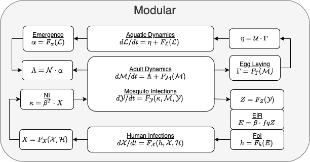
Figure 2