The Generalized Ross-Macdonald Adult Mosquito Model • exDE

The Generalized Ross-Macdonald adult mosquito model (GeRM) is a family of models that fulfills the generic interface of the adult mosquito component. A generalized version of the Ross-Macdonald model was first published in Spatial Dynamics of Malaria Transmission. Here, we present GeRM with exogenous forcing by resource availability. The state variables are: total mosquito density \(M\), gravid mosquito density \(G\), infected mosquito density \(Y\), and infectious mosquito density \(Z\).

In many ways, GeRM is similar to RM. A key difference is that in GeRM, it is possible to model bionomic models as a functional response to availability of resources. The parameterization is flexible, so that it is possible to simply pass the parameters as static values. Here, we illustrate with the standard parameterization.

Differential Equations

Delay Differential Equations

These equations are naturally implemented by exDE::dMYZdt.RM_dde, but they can also be implemented in a closely related set of odes using exDE::dMYZdt.RM_ode (see below).

\[ \dot{M} = \Lambda - \Omega\cdot M \] \[ \dot{G} = \mbox{diag}(f) \cdot (M-G) - \nu G - \Omega \cdot G \]

\[ \dot{Y} = \mbox{diag}(fq\kappa) \cdot (M-Y) - \Omega \cdot Y \]

\[ \dot{Z} = e^{-\Omega \tau} \cdot \mbox{diag}(fq\kappa_{t-\tau}) \cdot (M_{t-\tau}-Y_{t-\tau}) - \Omega \cdot Z \]

Recall that the mosquito demography matrix describing mortality and dispersal is given by:

\[ \Omega = \mbox{diag(g)} + \left(I- {\cal K}\right) \cdot \mbox{diag}(\sigma) \]

Ordinary Differential Equations

In the following, the equation are solved by exDE::dMYZdt.RM_ode.

The system of ODEs is the same as above except for the equation giving the rate of change in infectious mosquito density, which becomes:

\[ \dot{Z} = e^{-\Omega \tau} \cdot \mbox{diag}(fq\kappa) \cdot (M-Y) - \Omega \cdot Z \] The resulting set of equations is similar in spirit to the simple model presented in Smith & McKenzie (2004) in that mortality and dispersal over the EIP is accounted for, but the time lag is not. While transient dynamics of the ODE model will not equal the DDE model, they have the same equilibrium values, and so for numerical work requiring finding equilibrium points, the faster ODE model can be safely substituted.

Equilibrium solutions

There are two logical ways to begin solving the non-trivial equilibrium. The first assumes \(\Lambda\) is known, which implies good knowledge of mosquito ecology. The second assumes \(Z\) is known, which implies knowledge of the biting rate on the human population. We show both below.

Starting with \(\Lambda\)

Piven \(\Lambda\) we can solve:

\[ M = \Omega^{-1} \cdot \Lambda \] Then given \(M\) we set \(\dot{Y}\) to zero and factor out \(Y\) to get:

\[ Y = (\mbox{diag}(fq\kappa) + \Omega)^{-1} \cdot \mbox{diag}(fq\kappa) \cdot M \] We set \(\dot{Z}\) to zero to get:

\[ Z = \Omega^{-1} \cdot e^{-\Omega \tau} \cdot \mbox{diag}(fq\kappa) \cdot (M-Y) \]

Because the dynamics of \(P\) are independent of the infection dynamics, we can solve it given \(M\) as:

\[ G = (\Omega + \mbox{diag}(f+\nu))^{-1} \cdot \mbox{diag}(f) \cdot M \]

Starting with \(Z\)

It is more common that we start from an estimate of \(Z\), perhaps derived from an estimated EIR (entomological inoculation rate). Piven \(Z\), we can calculate the other state variables and \(\Lambda\). For numerical implementation, note that \((e^{-\Omega\tau})^{-1} = e^{\Omega\tau}\).

\[ M-Y = \mbox{diag}(1/fq\kappa) \cdot (e^{-\Omega\tau})^{-1} \cdot \Omega \cdot Z \]

\[ Y = \Omega^{-1} \cdot \mbox{diag}(fq\kappa) \cdot (M-Y) \]

\[ M = (M - Y) + Y \]

\[ \Lambda = \Omega \cdot M \] We can use the same equation for \(G\) as above.

Example

library(exDE)
library(expm)
library(deSolve)
library(data.table)
library(ggplot2)

Here we show an example of starting and solving a model at equilibrium. Please note that this only runs this adult mosquito model and that most users should read our fully worked example to run a full simulation.

nPatches <- 3
params <- make_parameters_xde("ode")
params$nPatches <- nPatches
params$nVectors =1

The Ross-Macdonald Parameterization

As with the RM model, we can set up the parameters for a simulation with 3 patches.

f <- 0.3
q <- 0.9
g <- 1/20
sigma <- 1/10
eip <- 11
nu <- 1/2
eggsPerBatch <- 30

calK <- matrix(0, nPatches, nPatches)
calK[1, 2:3] <- c(0.2, 0.8)
calK[2, c(1,3)] <- c(0.5, 0.5)
calK[3, 1:2] <- c(0.7, 0.3)
calK <- t(calK)

Omega <- make_Omega(g, sigma, calK, nPatches)
Upsilon <- expm::expm(-Omega * eip)

params = make_parameters_MYZ_GeRM(params, g, sigma, f, q, nu, eggsPerBatch, eip, calK, solve_as = "ode")

Now we set the values of \(\kappa\) and \(\Lambda\) and solve for the equilibrium values.

kappa <- c(0.1, 0.075, 0.025)
Lambda <- c(5, 10, 8)

Omega_inv <- solve(Omega)

M_eq <- as.vector(Omega_inv %*% Lambda)
G_eq <- as.vector(solve(diag(f+nu, nPatches) + Omega) %*% diag(f, nPatches) %*% M_eq)
Y_eq <- as.vector(solve(diag(f*q*kappa) + Omega) %*% diag(f*q*kappa) %*% M_eq)
Z_eq <- as.vector(Omega_inv %*% Upsilon %*% diag(f*q*kappa) %*% (M_eq - Y_eq))

We use exDE::make_inits_MYZ_RM to store the initial values. These equations have been implemented to compute \(\Upsilon\) dynamically, so we attach Upsilon as initial values:

params = make_inits_MYZ_GeRM_ode(pars = params, 
                             M0 = M_eq, G0 = G_eq, Y0 = Y_eq, Z0 = Z_eq)
params$Lambda[[1]] = Lambda 
params$kappa[[1]] = kappa

We and set the indices with exDE::make_indices.

params = make_indices(params)

Then we can set up the initial conditions vector and use deSolve::ode to solve the model. Normally these values would be computed within exDE::xDE_diffeqn. Here, we set up a local version:

y0 = get_inits_MYZ(params, 1) 


dMYZdt_local = function(t, y, pars, s=1) {
  list(dMYZdt(t, y, pars, s))
}

out <- deSolve::ode(y = y0, times = 0:50, dMYZdt_local, parms=params, 
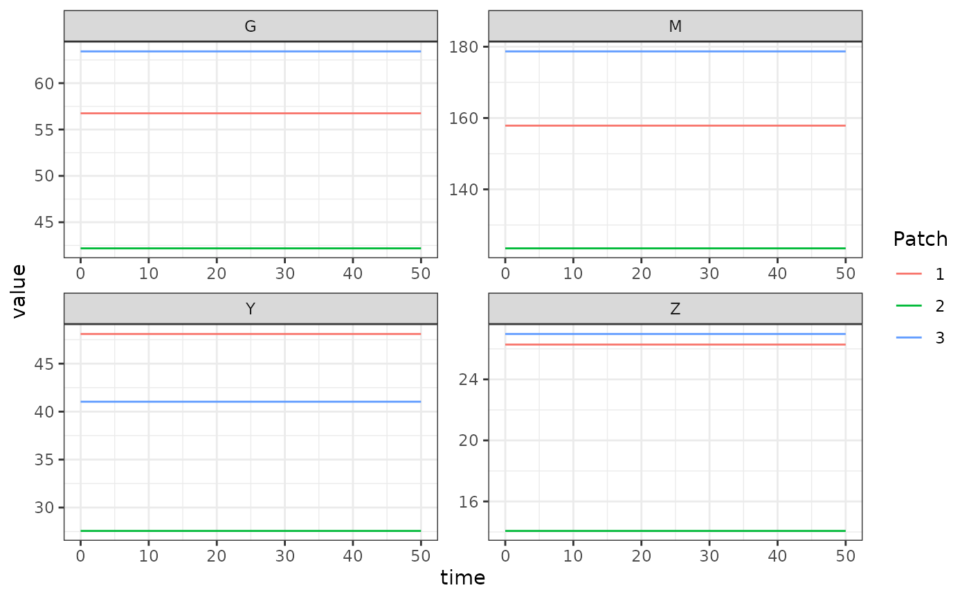
                    method = 'lsoda', s=1)

The output is plotted below. The flat lines shown here is a verification that the steady state solutions that we computed above match the steady states computed by solving the equations:

colnames(out)[params$ix$MYZ[[1]]$M_ix+1] <- paste0('M_', 1:params$nPatches)
colnames(out)[params$ix$MYZ[[1]]$G_ix+1] <- paste0('G_', 1:params$nPatches)
colnames(out)[params$ix$MYZ[[1]]$Y_ix+1] <- paste0('Y_', 1:params$nPatches)
colnames(out)[params$ix$MYZ[[1]]$Z_ix+1] <- paste0('Z_', 1:params$nPatches)

out <- as.data.table(out)
out <- melt(out, id.vars = 'time')
out[, c("Component", "Patch") := tstrsplit(variable, '_', fixed = TRUE)]
out[, variable := NULL]

ggplot(data = out, mapping = aes(x = time, y = value, color = Patch)) +
  geom_line() +
  facet_wrap(. ~ Component, scales = 'free') +
  theme_bw()