The SIS (Susceptible-Infected-Susceptible) human model model fulfills the generic interface of the human population component. It is the simplest model of endemic diseases in humans.
Differential Equations
We subdivide a population into susceptible (\(S\)) and infected and infectious (\(I\)) individuals, where the total population is \(H = S+I.\) We assume the force of infection (\(h\), FoI) is linearly proportional to the EIR: \(h = b \times EIR.\) In its general form, with births (\(B(H)\)) and deaths (at the per-capita rate \(\mu\)), the generalized SIS dynamics are:
\[ \begin{array}{rl} \dot{S} &= -h S + rI + B(H) -\mu S\\ \dot{I} &= h S - rI - \mu I \end{array} \]
If there is no demographic change, the SIS model can be rewritten as a single equation:
\[
\dot{I} = h (H-I) - rI
\] Even in this simplified form, we are assuming that a
population could be stratified, such that the variables and parameter
are all vectors with length nStrata.
Equilibrium Solutions
A typical situation when using this model is that \(H\) (total population size by strata) and \(X\) (number of infectious persons by strata) are known from census and survey data. Then it is of interest to find the value of \(EIR\) (Entomological Inoculation Rate) which leads to that prevalence at equilibrium.
\[ 0 = \mbox{diag}(bEIR) \cdot (H-I) - rI \]
\[ rI = \mbox{diag}(b) \cdot \mbox{diag}(EIR) \cdot (H-I) \]
\[ \frac{rI}{H-I} = \mbox{diag}(b) \cdot \mbox{diag}(EIR) \]
\[ \mbox{diag}(1/b) \cdot \left(\frac{rI}{H-I}\right) = EIR \]
Note that in the final line, \(EIR\) is a column vector of dimension \(n\) due to the operations on the left. Each element gives the per-capita rate at which individuals in that population strata receive potentially infectious bites (summing across all the places they visit).
Example
Here we run a simple example with 3 population strata at equilibrium.
We use exDE::make_parameters_X_SIS to set up parameters.
Please note that this only runs the human population component and that
most users should read our fully worked
example to run a full simulation.
We use the null (constant) model of human demography (\(H\) constant for all time).
The Long Way
To set up systems of differential equations, we must set the values of all our parameters.
nStrata <- 3
H <- c(100, 500, 250)
residence <- rep(1,3)
searchWtsH <- rep(1,3)
I <- c(20, 120, 80)
b <- rep(0.55, nStrata)
c <- rep(0.15, nStrata)
r <- rep(1/200, nStrata)
TaR <- matrix(data = 1,nrow = 1, ncol = nStrata)

EIR <- diag(1/b, nStrata) %*% ((r*I)/(H-I))
params <- make_parameters_xde()
params$nStrata = nStrata
params$nPatches = 1
params$nHosts = 1
params$eir = EIR
params$EIR = list()

fF_eir = function(EIR){
  EIR = as.vector(EIR)
  return(function(t, bday=0, scale=1){EIR})
}
F_eir = fF_eir(EIR)

params = make_parameters_demography_null(pars = params, H=H)

params = setup_BloodFeeding(params, 1, 1, residence=residence, searchWts=searchWtsH)
params$BFpar$TaR[[1]][[1]]=TaR

params = make_parameters_X_SIS(pars = params, b = b, c = c, r = r)

params = make_inits_X_SIS(pars = params, H-I, I)

params = make_indices(params)
y0 <- get_inits(params)

out <- deSolve::ode(y = y0, times = c(0, 365), xDE_diffeqn_cohort,
                    parms = params, method = 'lsoda', F_eir = F_eir)
out1 <- out
colnames(out)[params$ix$X$S_ix+1] <- paste0('S_', 1:params$nStrata)
colnames(out)[params$ix$X$I_ix+1] <- paste0('I_', 1:params$nStrata)

out <- as.data.table(out)
out <- melt(out, id.vars = 'time')
out[, c("Component", "Strata") := tstrsplit(variable, '_', fixed = TRUE)]
out[, variable := NULL]

ggplot(data = out, mapping = aes(x = time, y = value, color = Strata)) +
  geom_line() +
  facet_wrap(. ~ Component, scales = 'free') +
  theme_bw()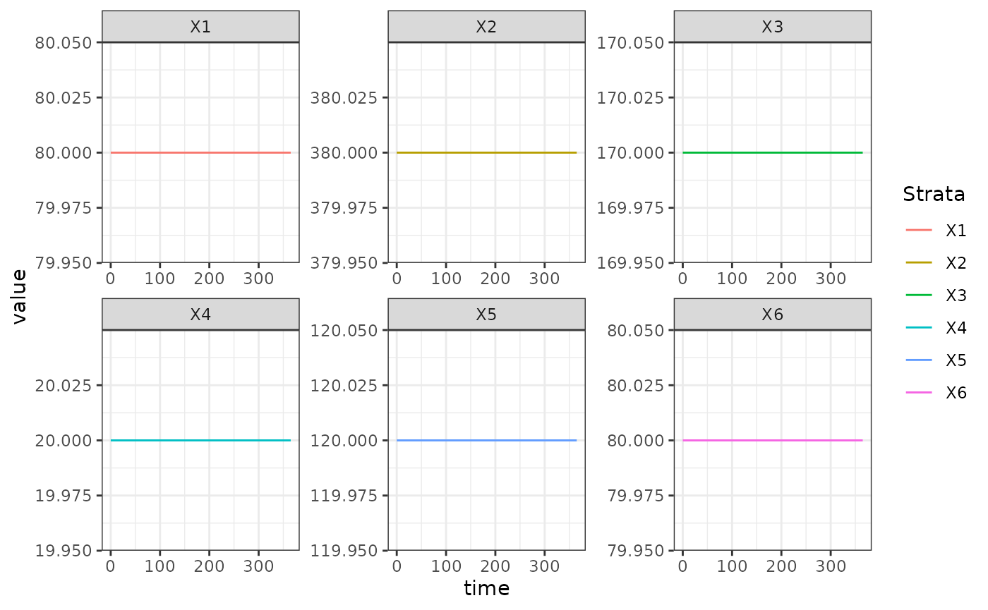
Using Setup
We have developed utilities for setting up models. We pass the parameter values and initial values as lists:
xde_setup_cohort(F_eir, Xname="SIS", HPop=Hpop, Xopts = Xo) -> test_SIS
xde_solve(test_SIS, 365, 365)$outputs$orbits$deout -> out2
approx_equal(out2,out1)
#>      time   X1   X2   X3   X4   X5   X6
#> [1,] TRUE TRUE TRUE TRUE TRUE TRUE TRUE
#> [2,] TRUE TRUE TRUE TRUE TRUE TRUE TRUE