The basic SIP (Susceptible-Infected-Prophylaxis) human model model fulfills the generic interface of the human population component. It is a reasonable first complication of the SIS human model. This requires two new parameters, \(\rho\), the probability a new infection is treated, and \(\eta\) the duration of chemoprophylaxis following treatment. \(X\) remains a column vector giving the number of infectious individuals in each strata, and \(P\) the number of treated and protected individuals.
Differential Equations
The equations are as follows:
\[ \dot{X} = \mbox{diag}((1-\rho)bEIR)\cdot (H-X-P) - (r+\xi)X \]
\[ \dot{P} = \mbox{diag}(\rho b EIR) \cdot (H-X-P) + \xi(H-P) - \eta P \]
Equilibrium solutions
Again, we assume \(H\) and \(X\) to be known, we set \(\xi=0\), and we solve for \(EIR\) and \(P\).
\[ P = \mbox{diag}(1/\eta) \cdot \mbox{diag}(\rho/(1-\rho)) \cdot rX \]
\[ EIR = \mbox{diag}(1/b) \cdot \mbox{diag}(1/(1-\rho)) \cdot \left( \frac{rX}{H-X-P} \right) \]
Given \(EIR\) we can solve for the mosquito population which would have given rise to those equilibrium values.
Example
Here we run a simple example with 3 population strata at equilibrium.
We use exDE::make_parameters_X_SIP to set up parameters.
Please note that this only runs the human population component and that
most users should read our fully worked
example to run a full simulation.
We use the null (constant) model of human demography (\(H\) constant for all time).
The Long Way
nStrata <- 3
H <- c(100, 500, 250)
residence <- rep(1,3)
searchWtsH <- rep(1,3)
I <- c(20, 120, 80)
b <- 0.55
c <- 0.15
r <- 1/200
eta <- c(1/30, 1/40, 1/35)
rho <- c(0.05, 0.1, 0.15)
xi <- rep(0, 3)
TaR <- matrix(data = 1,nrow = 1, ncol = nStrata)

P <- diag(1/eta) %*% diag(rho/(1-rho)) %*% (r*I)
EIR <- diag(1/b, nStrata) %*% diag(1/(1-rho)) %*% ((r*I)/(H-I-P))
params <- make_parameters_xde()
params$nStrata = nStrata
params$nPatches = 1
params$nHosts = 1

params$eir = EIR
params$EIR = list()

fF_eir = function(EIR){
  EIR = as.vector(EIR)
  return(function(t, bday=0, scale=1){EIR})
}
F_eir = fF_eir(EIR)

params = make_parameters_demography_null(pars = params, H=H)

params = setup_BloodFeeding(params, 1, 1, residence=residence, searchWts =searchWtsH)
params$BFpar$TaR[[1]][[1]]=TaR

params = make_parameters_X_SIP(pars = params, b = b, c = c, r = r, rho = rho, eta = eta, xi=xi)
params = make_inits_X_SIP(pars = params, H-I-P, I, as.vector(P))
params = make_indices(params)
y0 <- get_inits(params)
out <- deSolve::ode(y = y0, times = c(0, 365), xDE_diffeqn_cohort, parms = params, method = 'lsoda', F_eir = F_eir)
out1<- out
colnames(out)[params$ix$X[[1]]$S_ix+1] <- paste0('S_', 1:params$nStrata)
colnames(out)[params$ix$X[[1]]$I_ix+1] <- paste0('I_', 1:params$nStrata)
colnames(out)[params$ix$X[[1]]$P_ix+1] <- paste0('P_', 1:params$nStrata)

out <- as.data.table(out)
out <- melt(out, id.vars = 'time')
out[, c("Component", "Strata") := tstrsplit(variable, '_', fixed = TRUE)]
out[, variable := NULL]

ggplot(data = out, mapping = aes(x = time, y = value, color = Strata)) +
  geom_line() +
  facet_wrap(. ~ Component, scales = 'free') +
  theme_bw()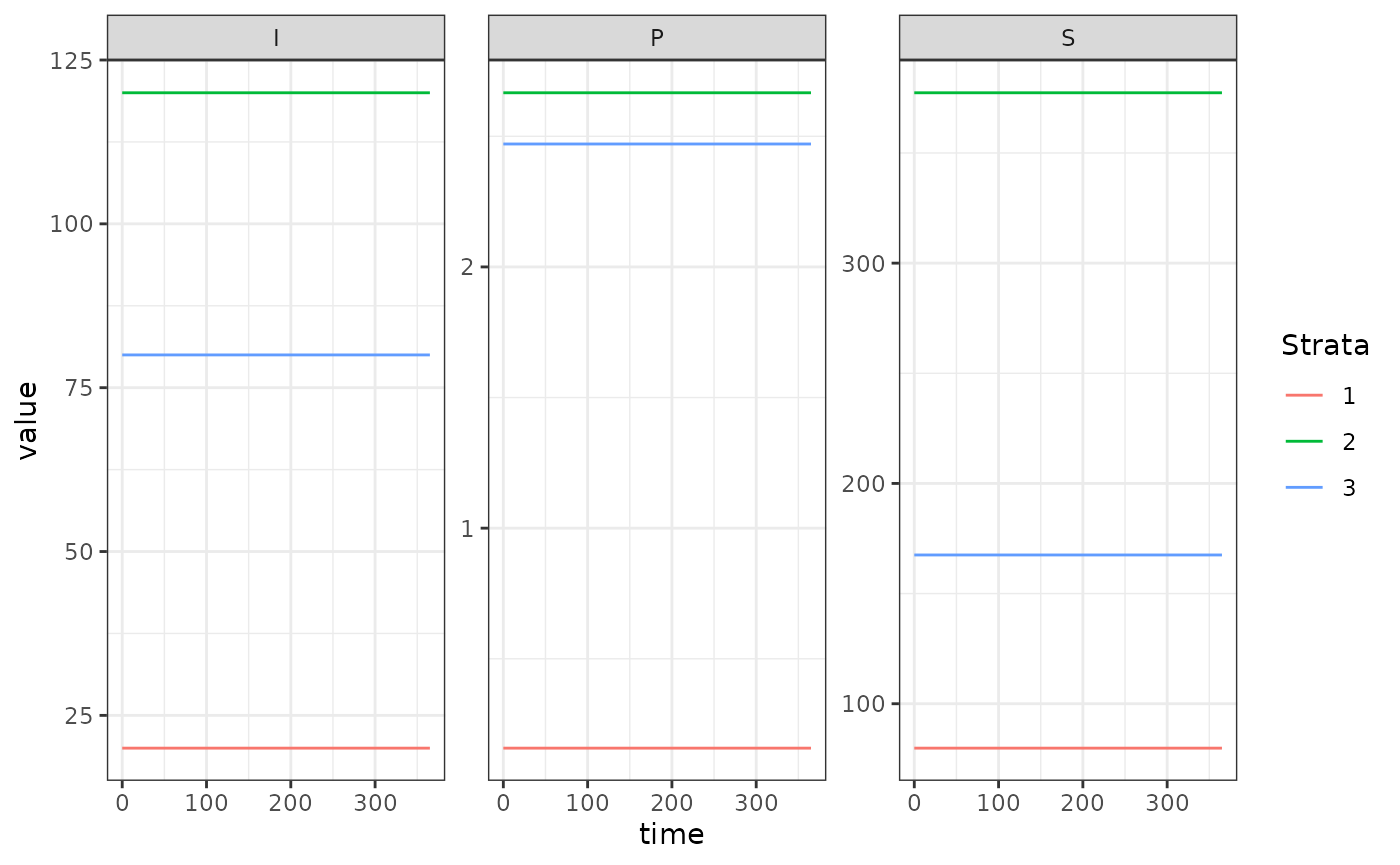
Using Setup
Xo = list(b=0.55, c=0.15, r=1/200,
          eta = c(1/30, 1/40, 1/35), rho = c(0.05, .1, 0.15),
          xi = rep(0,3),
          I0=I, P0=as.vector(P))
Hpop = c(100, 500, 250)
xde_setup_cohort(F_eir, Xname="SIP", HPop=Hpop, Xopts = Xo) -> test_SIP
xde_solve(test_SIP, 365, 365)$outputs$orbits$deout -> out2
approx_equal(out2,out1)
#>      time   X1   X2   X3   X4   X5   X6   X7   X8   X9
#> [1,] TRUE TRUE TRUE TRUE TRUE TRUE TRUE TRUE TRUE TRUE
#> [2,] TRUE TRUE TRUE TRUE TRUE TRUE TRUE TRUE TRUE TRUE