Hybrid MoI (Multiplicity of Infection) Human Model • exDE

This is a hybrid model which tracks the mean multiplicity of infection (superinfection) in two compartments. The first, $m1$ is all infections, and the second $m2$ are apparent (patent) infections. Therefore $m2$ is “nested” within $m1$ . It is a “hybrid” model in the sense of Nåsell (1985).

Differential Equations

The equations are as follows:

$\dot{m_{1}} = h - r_{1}m_{1}$ $\dot{m_{2}} = h - r_{2}m_{2}$ Where $h = b EIR$ , is the force of infection. Prevalence can be calculated from these MoI values by:

$x_{1} = 1-e^{-m_{1}}$ $x_{2} = 1-e^{-m_{2}}$ The net infectious probability to mosquitoes is therefore given by:

$x = c_{2}x_{2} + c_{1}(x_{1}-x_{2})$

Where $c_{1}$ is the infectiousness of inapparent infections, and $c_{2}$ is the infectiousness of patent infections.

Equilibrium solutions

One way to proceed is assume that $m_{2}$ is known, as it models the MoI of patent (observable) infections. Then we have:

$h = r_{2}/m_{2}$ $m_{1} = h/r_{1}$ We can use this to calculate the net infectious probability, and then $\kappa = \beta^{\top} \cdot x$ , allowing the equilibrium solutions of this model to feed into the other components.

Example

library(exDE)
library(deSolve)
library(data.table)
library(ggplot2)

Here we run a simple example with 3 population strata at equilibrium. We use exDE::make_parameters_X_hMoI to set up parameters. Please note that this only runs the human population component and that most users should read our fully worked example to run a full simulation.

We use the null (constant) model of human demography ( $H$ constant for all time). While $H$ does not appear in the equations above, it must be specified as the model of bloodfeeding ( $\beta$ ) relies on $H$ to compute consistent values.

The Long Way

Here, we build a model step-by-step.

nStrata <- 3
H <- c(100, 500, 250)
residence = rep(1,3) 
searchWtsH = rep(1,3) 
b <- 0.55
c1 <- 0.05
c2 <- 0.25
r1 <- 1/250
r2 <- 1/50
TaR <- matrix(data = 1, nrow = 1, ncol = nStrata)

m20 <- 1.5
h <- r2*m20
m10 <- h/r1

EIR <- rep(h/b, 3)

params <- make_parameters_xde()
params$nStrata = nStrata
params$nVectors = 1 
params$nHosts = 1
params$nPatches = 1 
params$EIR = list()

fF_eir = function(EIR){
  EIR = as.vector(EIR) 
  return(function(t, bday=0, scale=1){EIR})
} 
F_eir = fF_eir(EIR)

params = make_parameters_demography_null(pars = params, H=H) 

params = setup_BloodFeeding(params, 1, 1, residence=residence, searchWts=searchWtsH) 
params$BFpar$TaR[[1]][[1]]=TaR
params = make_parameters_X_hMoI(pars = params, b = b, c1 = c1, c2 = c2, r1 = r1, r2 = r2)
params = make_inits_X_hMoI(pars = params, rep(m10, nStrata), rep(m20, nStrata)) 
params = make_indices(params)

y0 <- get_inits(params)

out <- deSolve::ode(y = y0, times = c(0, 365), func = xDE_diffeqn_cohort, 
                    parms = params, method = 'lsoda', F_eir = F_eir) 
out1 <- out


colnames(out)[params$ix$X[[1]]$m1_ix+1] <- paste0('m1_', 1:params$nStrata)
colnames(out)[params$ix$X[[1]]$m2_ix+1] <- paste0('m2_', 1:params$nStrata)

out <- as.data.table(out)
out <- melt(out, id.vars = 'time')
out[, c("Component", "Strata") := tstrsplit(variable, '_', fixed = TRUE)]
out[, variable := NULL]

ggplot(data = out, mapping = aes(x = time, y = value, color = Strata)) +
  geom_line() +
  facet_wrap(Strata ~ Component, scales = 'free') +
  theme_bw()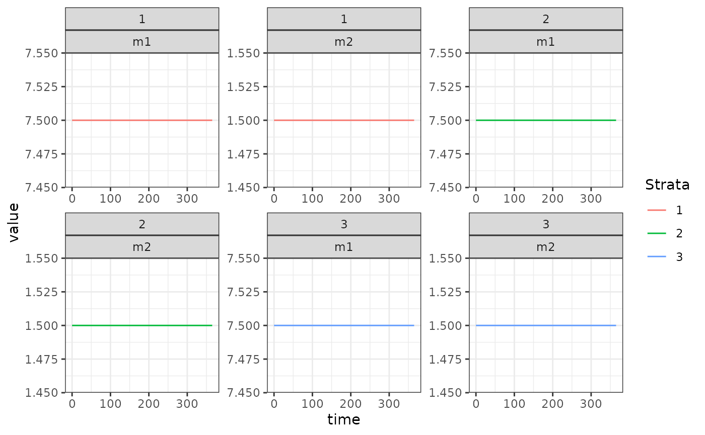

Using Setup

Xo = list(b=0.55, c1=0.05, c2=0.25, r1=1/250, r2=1/50, m20=1.5)
h = with(Xo, r2*m20) 
Xo$m10 = with(Xo, h/r1)  
Hpop = c(100, 500, 250)

xde_setup_cohort(F_eir, Xname="hMoI", HPop=Hpop, Xopts = Xo) ->test_hMoI

xde_solve(test_hMoI, 365, 365)$outputs$orbits$deout -> out2
approx_equal(out2, out1)
#>      time   X1   X2   X3   X4   X5   X6
#> [1,] TRUE TRUE TRUE TRUE TRUE TRUE TRUE
#> [2,] TRUE TRUE TRUE TRUE TRUE TRUE TRUE