Kernels

library(ramp.micro)

Point Sets

set.seed(24328)
bb = unif_xy(96, -17, 17) 
qq = unif_xy(89, -17, 17) 
ss = unif_xy(72, -17, 17)

Kernel Shapes

We use functions to generate the probability of finding a point as a function of its distance and context. Let $d_{i,j}$ denote the distance from point $i$ to $j$ . A scalar $\omega_j$ is a linear weight on each destination making it more or less attractive from every distance.

We define some function, $F_w$ that assigns a weight to every potential destination by distance. These weights are used to compute dispersal matrices (see below).

Exponential

The exponential family of functions has the following form

$\begin{equation} w_{j\rightarrow i} = F_w (d_{i,j}) = \omega_j e^{-k \left( \frac{d_{i,j}}{s}\right)^\gamma}. \end{equation}$

kFb = make_kF_exp(k=2, s=1, gamma=1.5)
kFq = make_kF_exp(k=2, s=2, gamma=2)
kFs = make_kF_exp(k=0.5, s=0.5, gamma=3)

dd = seq(0, 5, by = 0.01)
plot(dd, kFb(dd), type = "l", col = "darkred", xlab = "Distance", ylab = "Weight")
lines(dd, kFq(dd), type = "l", col = "darkblue")
lines(dd, kFs(dd), type = "l", col = "olivedrab4")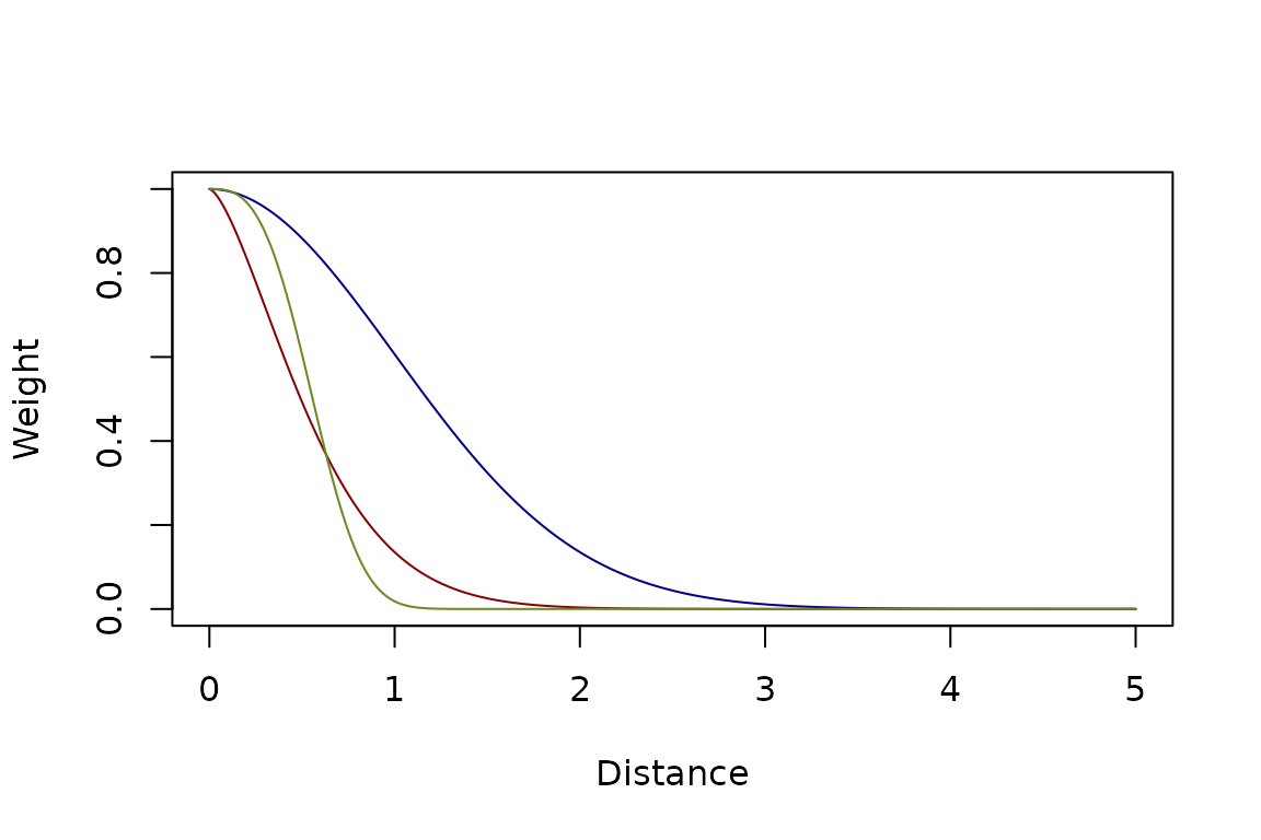

Power Law

Another function family for weight by distance is the distance raised to a power.

$\begin{equation} w_{j\rightarrow i} = F_w (d_{i,j}) = \frac{\omega_j}{(s+d_{i,j})^\delta}. \end{equation}$

kFb1 = make_kF_pwr(s=10, delta=1)
kFq1 = make_kF_pwr(s=1, delta=3)
kFs1 = make_kF_pwr(s=0.01, delta=2)

dd = seq(0, 5, by = 0.01)
plot(dd, kFb1(dd), type = "l", col = "darkred", xlab = "Distance", ylab = "Weight", ylim = c(0,1))
lines(dd, kFq1(dd), type = "l", col = "darkblue")
lines(dd, kFs1(dd), type = "l", col = "olivedrab4")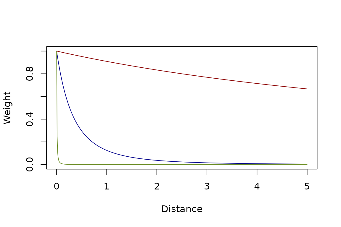

Mixture

The next function the sum of the two previous functions, where $\epsilon$ is the weight on each one of the functions.

$\begin{equation} w_{j\rightarrow i} = F_w (d_{i,j}) = \omega_j \left((1-p) e^{-k \left( \frac{d_{i,j}}{s_1}\right)^\gamma} + \frac{p}{(s_2+d_{i,j})^\delta} \right). \end{equation}$

Dispersal Matrices

Movement among point sets is modeled using matrices that describe where mosquitoes end up after dispersing in a single time step. The proportion moving from a point in one set to another, from $x\in \left\{ x \right\}$ to $y \in \left\{ y \right\}$ , is described by a matrix $\Psi_{y\leftarrow x}$ or equivalently $\Psi_{yx}$ . Similarly, the proportion moving from a point in one set to a point in the other is $\Psi_{xx}$ .

In translating distances into a probability mass function using the kernel shapes, we let

$w_{i,j} = F_w(d_{i,j})$ These weights are normalized and translated into proportions: the proportion arriving at each point in a destination set index by $j$ from a source set indexed by $i$ is normalized across all destinations from each starting point:

$\begin{equation} \Psi_{j,i} \in \Psi = \frac{w_{i,j}} {\sum_i w_{i,j}} \end{equation}$

Note that in the simulation models, these matrices describe the destinations for surviving mosquitoes, so we constrain the formulas such that each column sums to one. Mortality associated with dispersing is associated with the source points.

Blood Feeding

After emerging or after blood feeding, mosquitoes move from aquatic habitats to blood feed.

par(mar = c(1,1,2,2))
Psi_bq = make_Psi_xy(qq, bb, kFb, w=1)
plot_Psi_bq(bb, qq, Psi_bq)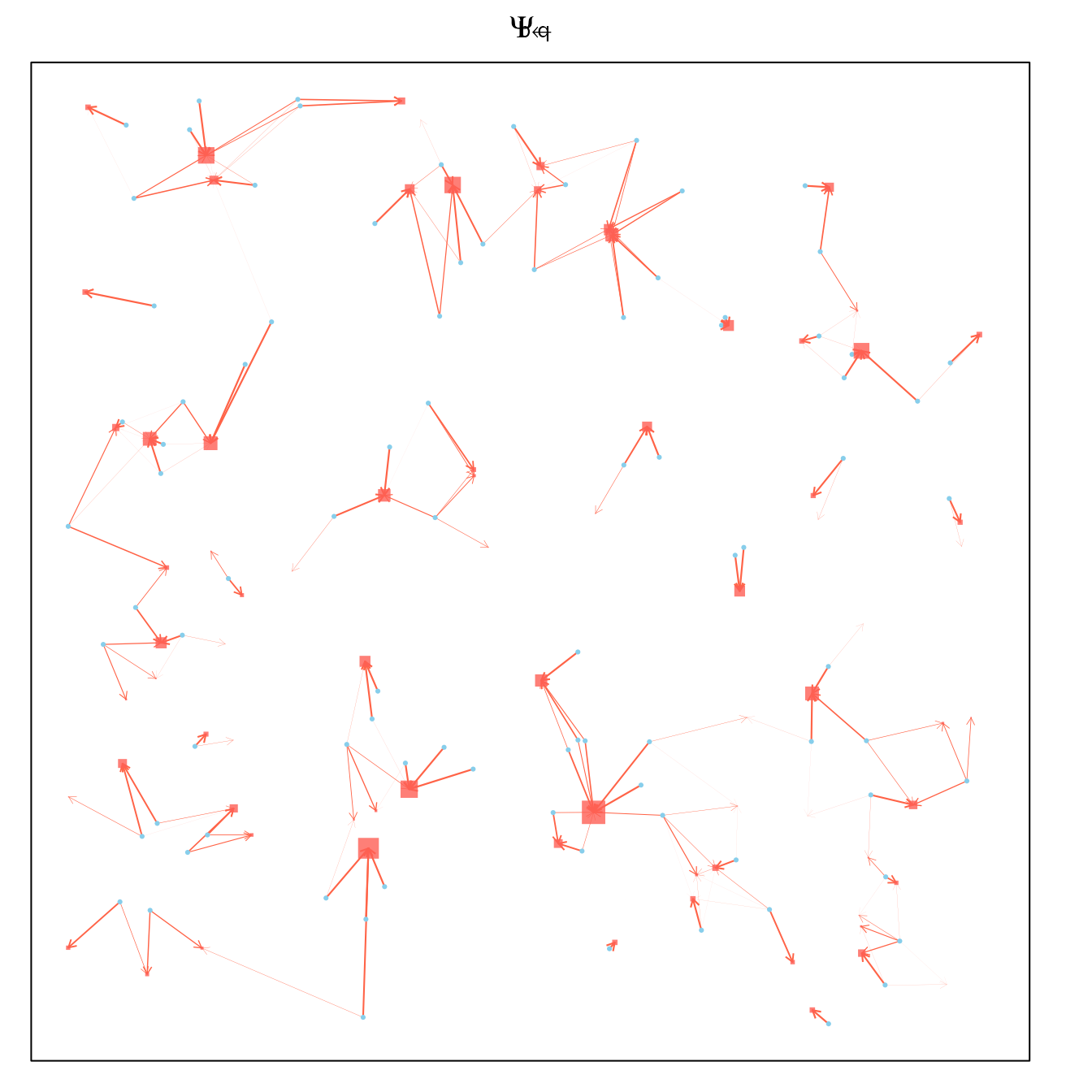

If they are unsuccessful, they will try to blood feed again. In the visualization, asymmetries arise because of the distribution of other points: $a$ and $b$ are close, and both are further away from $c$ so mosquitoes will tend to go back and forth between $a$ and $b$ and away from $c.$ The asymmetry is plotted by letting the colored portion of the arrow start

par(mar = c(1,1,2,2))
Psi_bb = make_Psi_xx(bb, kFb, w=1, stay=0.5)
plot_Psi_bb(bb, qq, Psi_bb)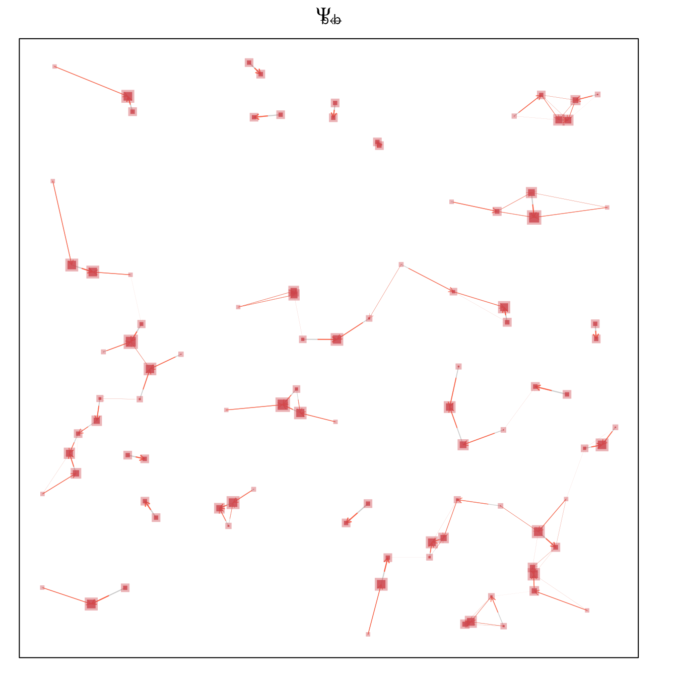

par(mar = c(1,1,2,2))
Psi_bs = make_Psi_xy(ss, bb, kFb, w=1)
plot_Psi_bs(bb, qq, ss, Psi_bs)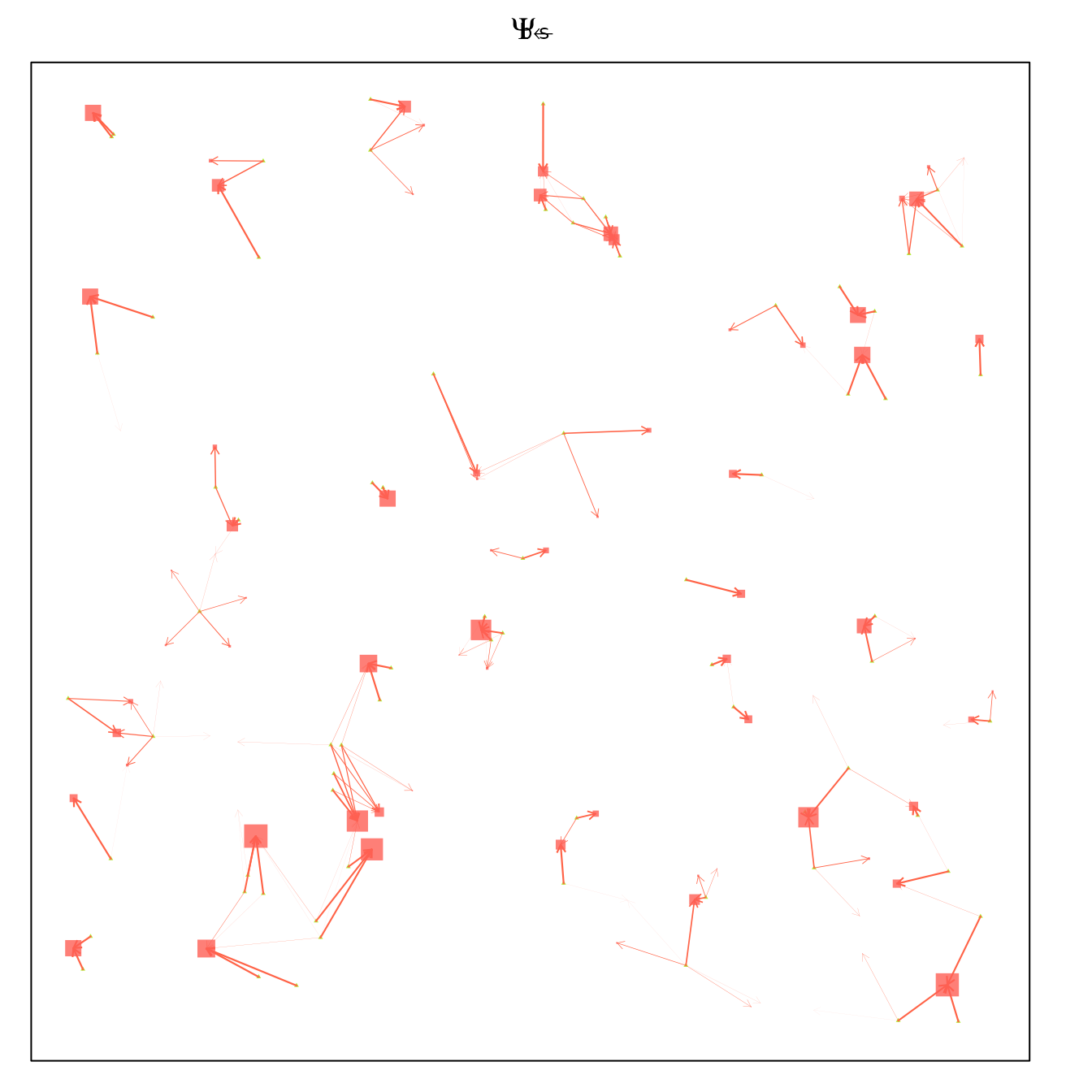

Egg Laying

After blood feeding, mosquitoes move from blood feeding sites to aquatic habitats.

par(mar = c(1,1,2,2))
Psi_qb = make_Psi_xy(bb, qq, kFb, w=1)
plot_Psi_qb(bb, qq, Psi_qb)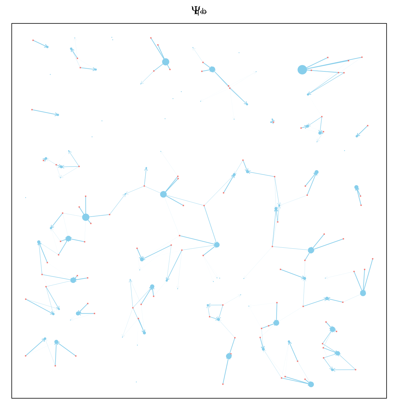

If they fail, mosquitoes will move again.

par(mar = c(1,1,2,2))
Psi_qq = make_Psi_xx(qq, kFq, w=1, stay=0.3)
plot_Psi_qq(bb, qq, Psi_qq)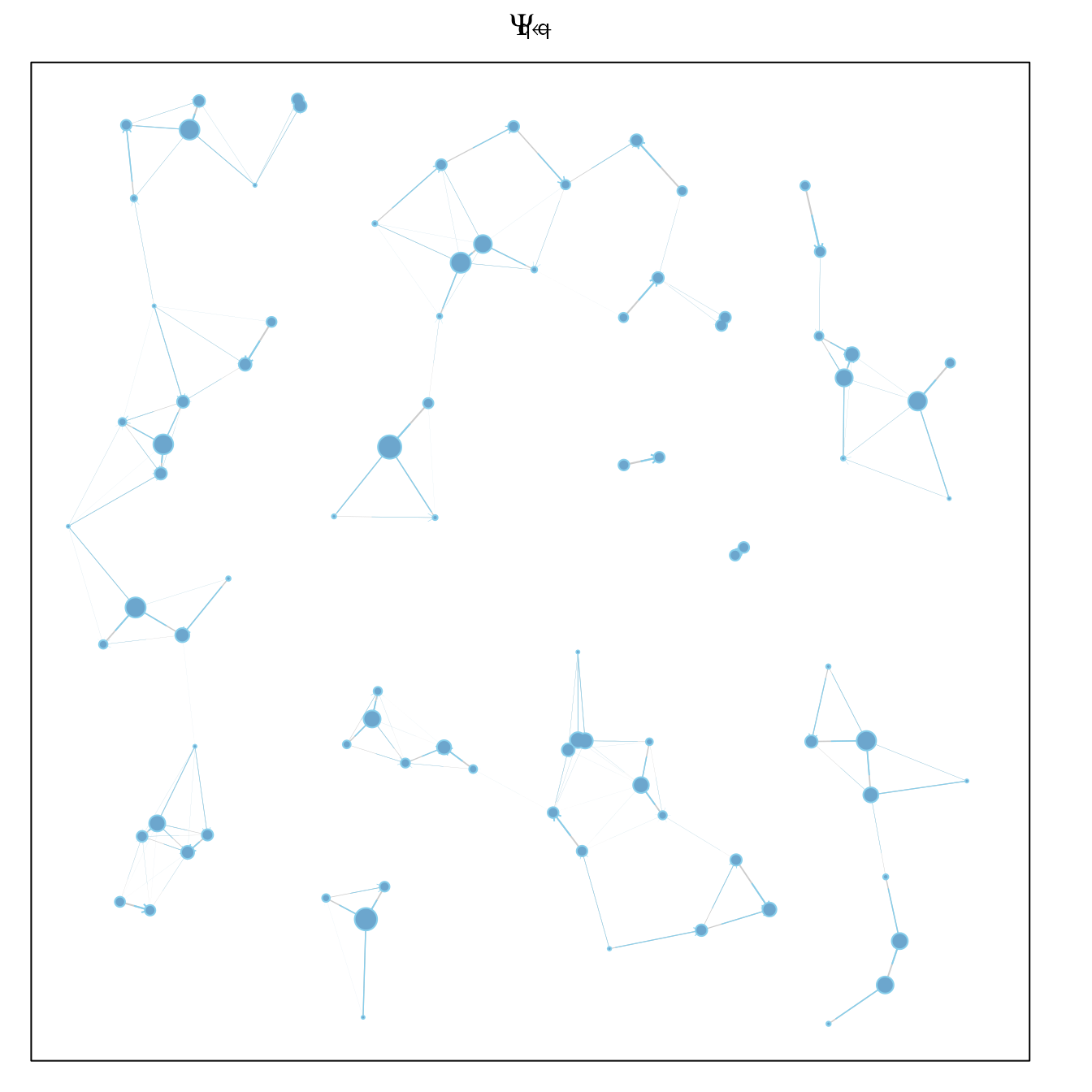

Sugar Feeding

par(mar = c(1,1,2,2))
Psi_sb = make_Psi_xy(bb, ss, kFs, w=1)
plot_Psi_sb(bb, qq, ss, Psi_sb)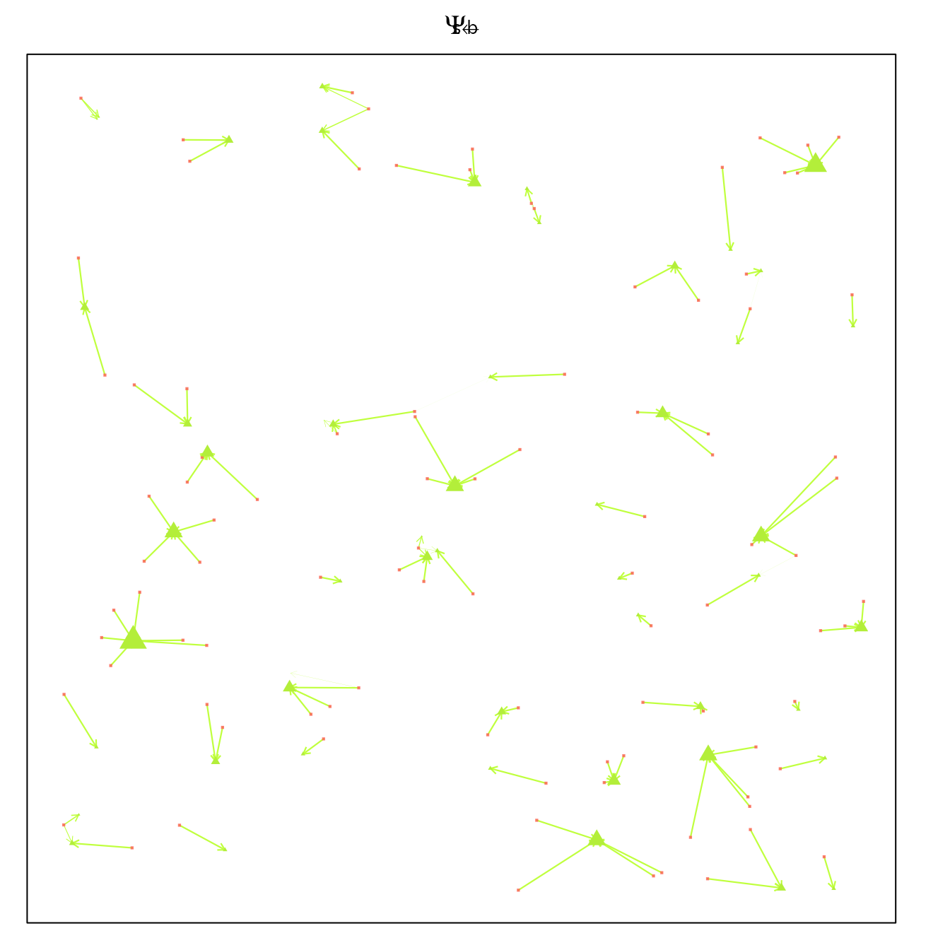

par(mar = c(1,1,2,2))
Psi_sq = make_Psi_xy(qq, ss, kFs, w=1)
plot_Psi_sq(bb, qq, ss, Psi_sq)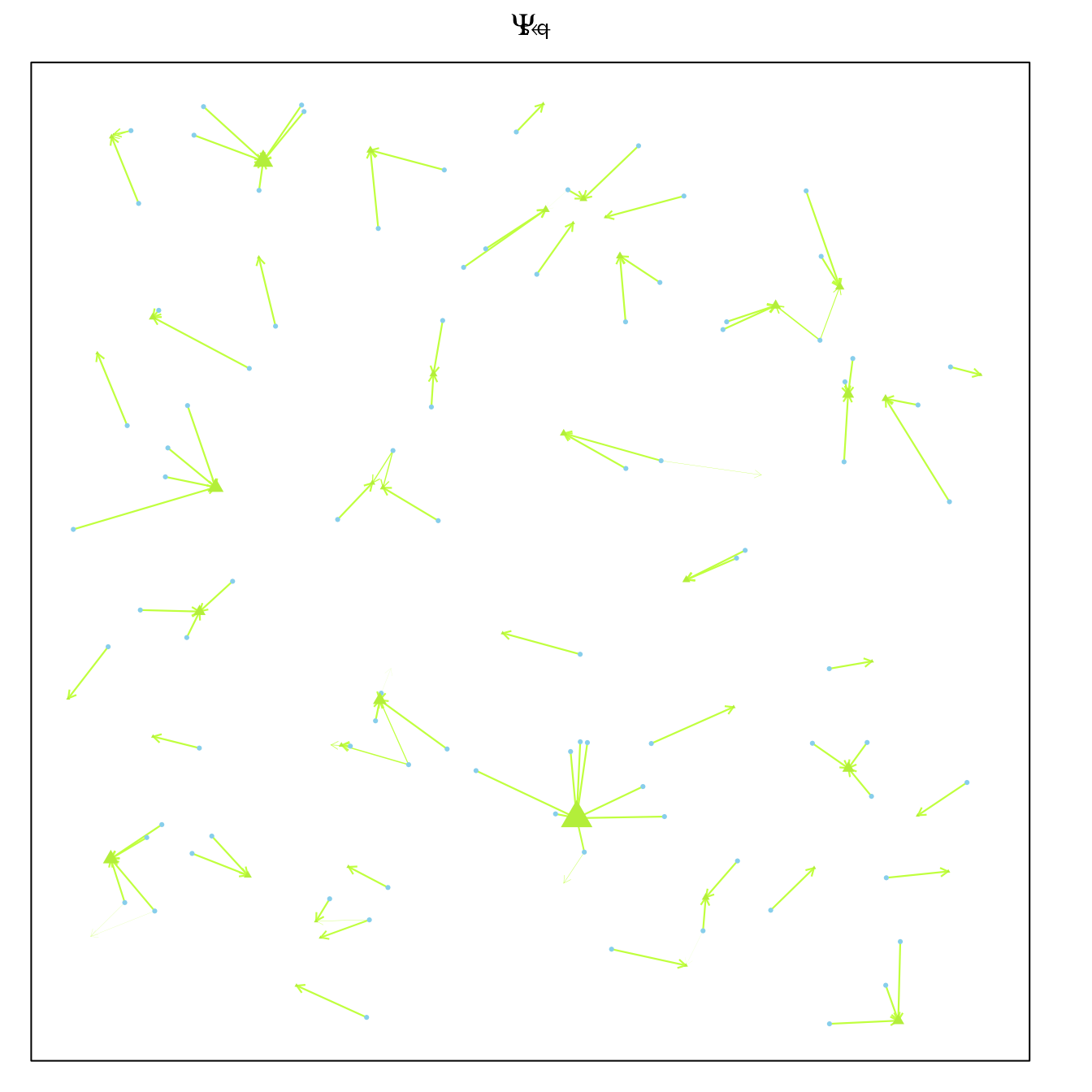

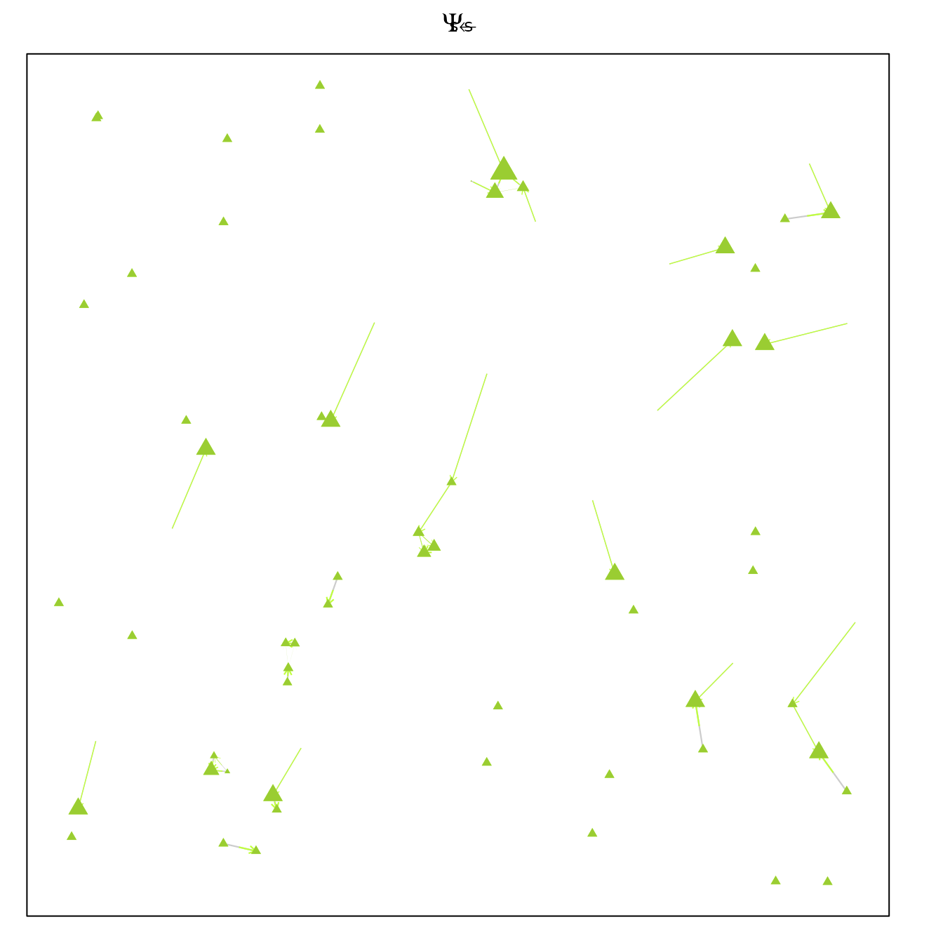
par(mar = c(1,1,2,2))
Psi_ss = make_Psi_xx(ss, kFs, w=1, stay=0.05)
plot_Psi_ss(bb, qq, ss, Psi_ss)

Setting Up Movement Matrices