Skip to contents

To quantify mosquito movement through one phase of the feeding cycle – either blood feeding or egg laying – that involves an initial search from another resource that could be followed by several failures, we developed a ``trap’’ algorithm that computes isolates one part of the feeding cycle.

To do so, we modify the simulation by setting to zero the parameters describing how mosquitoes would leave the trap state. We then initialize and follow a cohort from the point it enters that state, iterating until almost surviving mosquitoes accumulate in the end state (i.e., up to a predefined tolerance). We let KbqK_{b\leftarrow q} denote a |b|×|q||b| \times |q| matrix describing net dispersal to blood feed once: it is the proportion of mosquitoes leaving {q}\left\{q\right\} after laying eggs that eventually blood feed successfully at each point in {b}\left\{b\right\}. Similarly, we define KqbK_{q \leftarrow b} denote net dispersal to lay eggs after.

BQ Model

In the case of blood feeding, we begin with a cohort of mosquitoes in {q}\left\{q\right\} that has just successfully laid eggs. In the BQ model, all these mosquitoes launch in search of blood, some of them surviving to end up at a point in in {b}\left\{b\right\}:

B0=Ψbqdiag(pq) B_0 = \Psi_{b \leftarrow q} \cdot \mbox{diag}\left(p_q \right) B0B_0 is thus defined as a |b|×|q||b| \times |q| matrix.

Some of these will successfully blood feed, and we divert these into the trap state, T.T. It is initialized to zero but with the same shape as B0B_0:

T0=0B0 T_0 = 0 B_0 Now, we iterate until the sum of all elements in BtB_t is negligible, or Bt<ϵ\left\| B_t\right \| < \epsilon:

Tt+1=Tt+diag(ψb)BtBt+1=Ψbbdiag(pb(1ψb))Bt \begin{array}{rl} T_{t+1} &= T_t + \mbox{diag}\left(\psi_b \right) \cdot B_t \\ B_{t+1} &= \Psi_{b \leftarrow b} \cdot \mbox{diag}\left(p_b \left(1-\psi_b \right)\right) \cdot B_t \\ \end{array} So that Kbq=limtTt.K_{b\leftarrow q} = \lim_{t \rightarrow \infty} T_t.

In the BQ model, we can use the same idea to compute Kqb.K_{q \leftarrow b}. These are the functions compute_Kqb.BQ and compute_Kbq.BQ

BQS Model

KbqK_{b \leftarrow q}

Q0=diag(pq) Q_0 = \mbox{diag}\left(p_q \right)

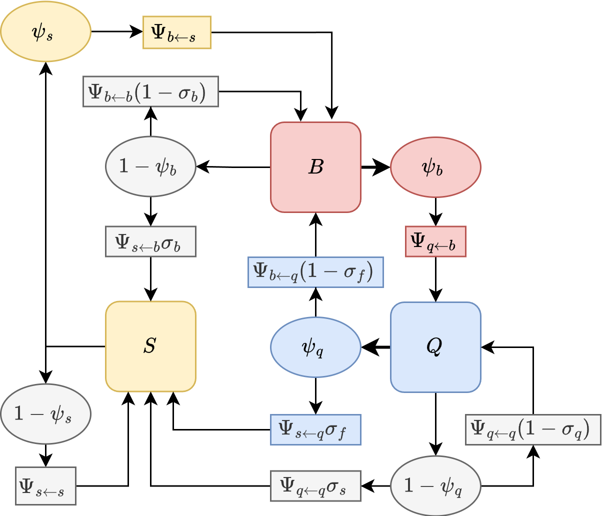
In the BQS model, we start out the same way, but after leaving {q},\left\{q\right\}, the trap is set at the end of blood feeding; since a blood meal is required to lay eggs, there are no transitions back to egg laying.

B0=Ψbqdiag((1σf))Q0S0=Ψsqdiag(σf)Q0T0=0B0 \begin{array}{rl} B_0 &= \Psi_{b \leftarrow q} \cdot \mbox{diag}\left((1-\sigma_f) \right) \cdot Q_0 \\ S_0 &= \Psi_{s \leftarrow q} \cdot \mbox{diag}\left(\sigma_f \right) \cdot Q_0 \\ T_0 &= 0 B_0 \\ \end{array}

Thereafter, we can compute the state transitions. Abusing notation a bit (we let []\left[ \right] indicate diag()\mbox{diag}\left(\right)), Since no transitions back to QQ are possible, the trap matrix is:

[Bt+1St+1Tt+1]=[Ψbb[(1σb)pb(1ψb)]Ψbs[psψs]0Ψsb[σbpb(1ψb)]Ψss[ps(1ψs)]0[ψb]0[1]][BtStTt] \begin{equation}\begin{array}{l} \left[ \begin{array}{c} B_{t+1} \\ S_{t+1} \\ T_{t+1} \\ \end{array} \right] = \left[ \begin{array}{ccc} \Psi_{bb} \cdot \left[\left(1-\sigma_b\right) p_b \ \left(1- \psi_b \right) \right] & \Psi_{bs} \cdot \left[p_s \psi_s \right] & 0 \\ \Psi_{sb} \cdot \left[\sigma_b p_b \left(1-\psi_b \right) \right] & \Psi_{ss}\cdot \left[p_s \left(1-\psi_s \right) \right] & 0 \\ \left[\psi_b \right] & 0 & \left[1 \right]\\ \end{array} \right] \left[ \begin{array}{c} B_t \\ S_t \\ T_t \end{array} \right] \end{array} \end{equation}

KqbK_{q \leftarrow b}

The trap model for egg laying after blood feeding is more complicated because an unsuccessful egg laying attempt could be followed by a sugar feeding attempt. In this model, the implication is that the mosquito has reabsorbed the eggs, and another blood meal is required.

B0=diag(pb) B_0 = \mbox{diag}\left(p_b \right)

Q0=0(ΨqbB0)S0=0(ΨbsB0)T0=0Q0 \begin{array}{rl} Q_0 & = 0 \left(\Psi_{qb} \cdot B_0 \right) \\ S_0 & = 0 \left(\Psi_{bs} \cdot B_0 \right) \\ T_0 & = 0 Q_0 \\ \end{array} and the calculation is:

[Bt+1Qt+1St+1Tt+1]=[Ψbb[((1σb)pb(1ψb))]0Ψbs[ψsps]0Ψqb[ψbpb]Ψqq[(1σq)pq(1ψq)]00Ψsb[σbpb(1ψb)]Ψsq[σqps(1ψq)]Ψss[1ψs]00[ψq]0[1]][BtQtStTt] \begin{equation}\begin{array}{l} \left[ \begin{array}{c} B_{t+1} \\ Q_{t+1} \\ S_{t+1} \\ T_{t+1} \\ \end{array} \right] = \left[ \begin{array}{ccc} \Psi_{bb} \cdot \left[\left((1-\sigma_b)p_b(1-\psi_b) \right)\right] & 0 & \Psi_{bs} \cdot \left[\psi_s p_s\right] & 0 \\ \Psi_{qb} \cdot \left[\psi_b p_b\right] & \Psi_{qq} \cdot \left[ (1-\sigma_q) p_q (1- \psi_q) \right]& 0 & 0 \\ \Psi_{sb} \cdot \left[\sigma_b p_b (1-\psi_b) \right] & \Psi_{sq} \cdot \left[\sigma_q p_s \left(1-\psi_q\right) \right]& \Psi_{ss} \cdot \left[1-\psi_s \right] & 0 \\ 0 & \left[\psi_q \right] & 0 & \left[1\right]\\ \end{array} \right] \left[ \begin{array}{c} B_t \\ Q_t \\ S_t \\ T_t \end{array} \right] \end{array} \end{equation}