A Workhorse Model for Human Infection

suppressMessages(library(knitr))
suppressMessages(library(ramp.xds))
#suppressMessages(library(ramp.library))
library(deSolve)
library(ramp.library)
#devtools::load_all()

Warning: workhorse is in development.

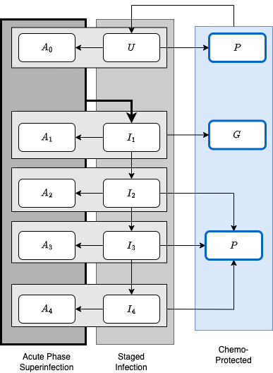
In the following, we present a stage of infection (SoI) model for malaria infection that recognizes an important difference between the two major phases of an infection: the acute phase characterized by geometrically increasing parasite numbers; and the chronic phase characterized by fluctuating parasite densities. The model explicitly considers superinfection, which moves individuals from an infected state into a parallel set of states.

Uninfected individuals are either susceptible to infection \(U\) or chemoprotected and not susceptible to infection.
Some recently treated, chemoprotected individuals remain infections \(G.\) The remainder are chemoprotected and not infectious, \(P.\)
There are four chronic infection stages.
There are five acute infection stages: four that correspond to an acute-phase infection concurrently infected with parasites in the chronic phase; and one that corresponds to carrying an acute phase infection but being otherwise uninfected.
All acutely infected individuals transition into \(I_1\)

Variables

The variables are thus:

\(U\)
Chemoprotected states are \(P\) and \(G\)

Active acute-phase infections become apparent after \(\tau\) days, and:

Uninfected

\[ \begin{array}{rl} \frac{dU}{da} &= r \sum_i I_i + \sigma (P + G) - (h_\tau + \zeta_U) U \\ \frac{dA_0}{da} &= r \sum_i A_i + h_\tau U - (\phi + \zeta_A + \zeta_U) A_0 \end{array} \] Chemoprotected

We are assuming that treatment as a result of an acute infection could leave a person infectious:

\[ \begin{array}{rl} \frac{dP}{da} &= \zeta_U (U + A_0) + \sum_{i\geq 2} \zeta_i I_i - \sigma P \\ \frac{dG}{da} &= \zeta_1 I_1 + \zeta_A \sum_i A_i - \sigma G \\ \end{array} \]

Infected

Where \(\phi\) is on the order of \(1/10 d\) and

At peak:

\[ \begin{array}{rl} \frac{dI_1}{da} & = p(w) \phi \sum_i A_i - (h_\tau + r + \xi_1 + \zeta_1) I_1 \\ \frac{dI_2}{da} & = (1-p(w)) \phi \sum_i A_i + \xi_1 I_1 - (h_\tau + r + \xi_2+ \zeta_2) I_2 \\ \frac{dI_3}{da} & = \xi_2 I_2 - (h_\tau + r + \xi_3 + \zeta_3) I_3 \\ \frac{dI_4}{da} & = \xi_3 I_3 - (h_\tau + r + \zeta_4) I_4 \\ \end{array} \]

Past peak, for \(n \in 2,3,4\):

\[ \begin{array}{rl} \frac{dA_1}{da} & = h_\tau I_1 - \phi A_1 - (\zeta_A + r + \zeta_1) A_1 \\ \frac{d A_n}{da} &= h_\tau I_n - \phi A_n - (\zeta_A + \zeta_n) I_n\\ \end{array} \] Immune Tracking

\[ \begin{array}{rl} \frac{d w_0}{da} &= h_\tau \\ \frac{d w_i}{da} &= h_\tau - \delta_I w_i \\ \end{array} \]

#devtools::load_all()

wh <- xds_setup(Xname = "workhorse", 
                HPop=1000,
                Lname = "trivial", 
                Lopts = list(
                  Lambda = 3000, 
                  F_season = function(t){1+sin(2*pi*t/365)}
                  )
                )

wh <- xds_solve(wh, Tmax = 5*365, dt=10)

wh1 = wh 
wh1$Xpar[[1]]$zeta_1 = 0.02
wh1 <- xds_solve(wh1, Tmax = 5*365, dt=10)

xds_plot_X(wh)
xds_plot_X(wh1, llty=2, add_axes=FALSE)

with(wh$outputs$orbits$XH[[1]],{
  A = A0+A1+A2+A3+A4
  I = I1+I2+I3+I4
  plot(time, U + P + G, type = "l", ylim = range(0, H), col = "darkblue") 
  lines(time, A+I, col = "darkred") 
  lines(time, A, col = "purple") 
  lines(time, I-I1, col = "orange") 
  lines(time, P+G, col = "darkgreen") 
})

with(wh1$outputs$orbits$XH[[1]],{
  A = A0+A1+A2+A3+A4
  I = I1+I2+I3+I4
  lines(time, U + P + G, col = "darkblue", lty=2) 
  lines(time, A+I, col = "darkred", lty=2) 
  lines(time, A, col = "purple", lty=2) 
  lines(time, I-I1, col = "orange", lty=2) 
  lines(time, P+G, col = "darkgreen", lty=2) 
})

September 07, 2024

Variables