SIP_xde (Susceptible-Infected-Prophylaxis) Human Model • ramp.library

The basic SIP_xde (Susceptible-Infected-Prophylaxis) human model model fulfills the generic interface of the human population component. It is a reasonable first complication of the SIS human model. This requires two new parameters, $\rho$ , the probability a new infection is treated, and $\eta$ the duration of chemoprophylaxis following treatment. $X$ remains a column vector giving the number of infectious individuals in each strata, and $P$ the number of treated and protected individuals.

Differential Equations

The equations are formulated around the FoI, $h$ . Under the default model, we get the relationship $h = b E$ , where $E$ is the daily EIR:

$\frac{dI}{dt} = h (1-\rho) (H-I-P) - (r+\xi)I$

$\frac{dP}{dt} = h \rho \cdot (H-I-P) + \xi(H-P) - \eta P$

Equilibrium solutions

We can compute the steady states as a function of the FoI, $h$ :

$\bar I = H \frac{h \eta (1-\rho)}{(h+r+\xi)(\eta+\xi) +h(r-\eta)\rho}$ and

$\bar P = H\frac{\xi(h+r+\xi) + hr\rho}{(h+r+\xi)(\eta+\xi) +h(r-\eta)\rho}$ and $\bar S = H - \bar I - \bar P$

Example

library(ramp.xds)
library(ramp.library)
library(deSolve)
library(data.table)
library(ggplot2)

Here we run a simple example with 3 population strata at equilibrium. We use ramp.xds::make_parameters_X_SIP_xde to set up parameters. Please note that this only runs the human population component and that most users should read our fully worked example to run a full simulation.

We use the null (constant) model of human demography ( $H$ constant for all time).

The Long Way

nStrata <- 3
H <- c(100, 500, 250)
nPatches <- 3
residence <- 1:3 
params <- make_xds_template("ode", "human", nPatches, 1, residence)

b <- 0.5
c <- 0.15
r <- 1/200
eta <- c(1/30, 1/40, 1/35)
rho <- c(0.05, 0.1, 0.15)
xi <- rep(0, 3)
Xo = list(b=b,c=c,r=r,eta=eta,rho=rho,xi=xi)
class(Xo) <- "SIP"

eir <- c(1,2,3)/365
xde_steady_state_X(eir*b, H, Xo) ->ss
ss
#> $H
#> [1] 100 500 250
#> 
#> $I
#> [1]  20.61856 163.93443 101.53295
#> 
#> $P
#> [1] 0.1627781 3.6429872 3.1355763

Xo$I <- ss$I
Xo$P <- ss$P

params = setup_Xpar("SIP", params, 1, Xo) 
params = setup_Xinits(params, H, 1, Xo)

MYZo = list(
  Z = eir*H, f=1, q=1
)

params = setup_MYZpar("trivial", params, 1, MYZo)
params = setup_MYZinits(params, 1)
params <- setup_Hpar_static(params, 1)
params = setup_Lpar("trivial", params, 1)
params = setup_Linits(params, 1)

params = make_indices(params)

xde_steady_state_X(eir*b, H, params$Xpar[[1]])
#> $H
#> [1] 100 500 250
#> 
#> $I
#> [1]  20.61856 163.93443 101.53295
#> 
#> $P
#> [1] 0.1627781 3.6429872 3.1355763

y0 <- as.vector(unlist(get_inits(params)))

out <- deSolve::ode(y = y0, times = c(0, 730), xde_derivatives, parms= params, method = 'lsoda') 
list_Xvars(out, params, 1)
#> $S
#> [1] -350.0000  -20.0000 -420.6186
#> 
#> $I
#> [1] 100 500 500
#> 
#> $P
#> [1] 250.00000 250.00000  20.61856
#> 
#> $H
#> [1]   0 730 100

colnames(out)[params$ix$X[[1]]$H_ix+1] <- paste0('H_', 1:params$nStrata)
colnames(out)[params$ix$X[[1]]$I_ix+1] <- paste0('I_', 1:params$nStrata)
colnames(out)[params$ix$X[[1]]$P_ix+1] <- paste0('P_', 1:params$nStrata)

out <- as.data.table(out)
out <- melt(out, id.vars = 'time')
out[, c("Component", "Strata") := tstrsplit(variable, '_', fixed = TRUE)]
out[, variable := NULL]

ggplot(data = out, mapping = aes(x = time, y = value, color = Strata)) +
  geom_line() +
  facet_wrap(. ~ Component, scales = 'free') +
  theme_bw()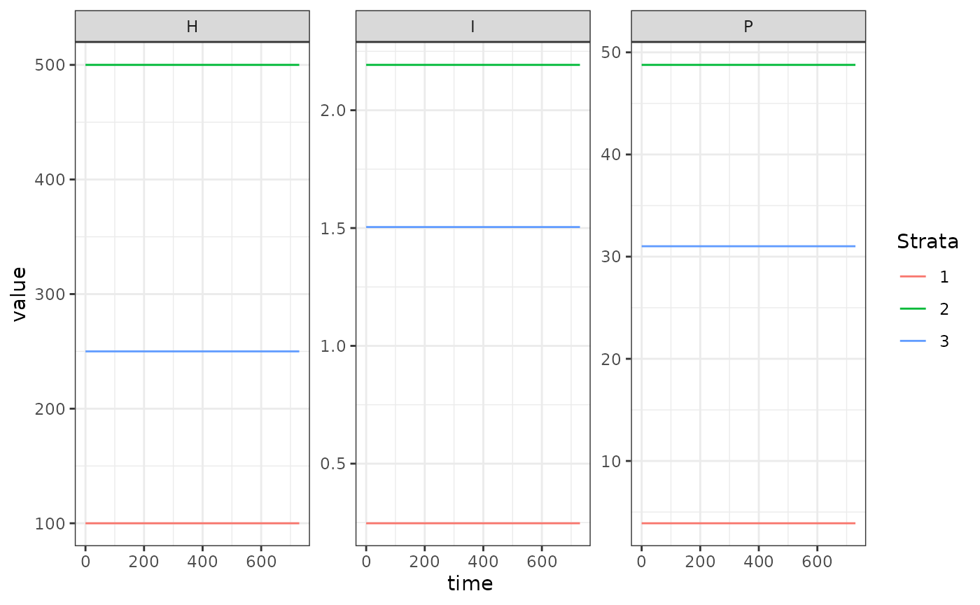

Using Setup

xds_setup_human(Xname="SIP", nPatches=3, residence = 1:3, HPop=H, Xopts = Xo, MYZopts = MYZo) -> test_SIP_xde

xde_steady_state_X(b*eir, H, test_SIP_xde$Xpar[[1]]) -> out1
out1 <- unlist(out1)

xds_solve(test_SIP_xde, 365, 365)$outputs$last_y -> out2
approx_equal(out2,out1) 
#>      [,1] [,2] [,3] [,4] [,5] [,6] [,7] [,8] [,9]
#> [2,] TRUE TRUE TRUE TRUE TRUE TRUE TRUE TRUE TRUE