Hybrid Model for the Age of Infection

Hybrid Model

The function solve_dAoI computes the first three moments of the AoI by default. Here we plot the $n^{th}$ root of the first three moments.

par(mar = c(7, 4, 2, 2))
solve_dAoI(5/365, foiP3) -> mt 
plot(mt$time, mt$xn1, type = "l", xlab = "Age (in Days)", ylab = expression(list(x, sqrt(x[paste("[2]")]), sqrt(x[paste("[3]")], 3))), ylim = range(mt$xn3^(1/3))) 
lines(mt$time, mt$xn2^(1/2), col = "purple")
lines(mt$time, mt$xn3^(1/3), col = "darkgreen")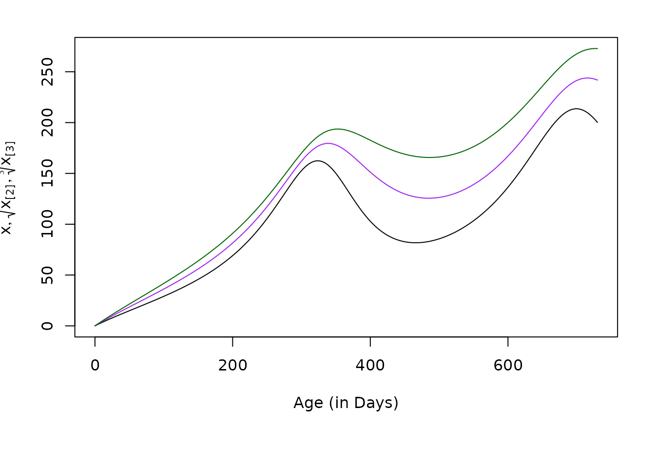 

## Numerical Verification

aa = seq(1, 5*365, by = 5) 
moment1 = momentAoI(aa, foiP3)
moment2 = momentAoI(aa, foiP3, n=2)
moment3 = momentAoI(aa, foiP3, n=3)

2. By solving a hybrid model with variables that track the moments, using the equations that we derived above:

solve_dAoI(5/365, foiP3, Tmax = 5*365, dt=5) -> mt 

par(mfrow = c(2,2), mar = c(7, 4, 2, 2))
# Top Left
plot(mt$time, mt$xn1, type = "l", xlab = "Age (in Days)", ylab = expression(x), lwd=3) 
lines(aa, moment1, col = "yellow", lwd=2, lty=2) 
# Top Right 
plot(mt$time, mt$xn2, type = "l", xlab = "Age (in Days)", ylab = expression(x[paste("[2]")]), lwd=3, col = "purple") 
lines(aa, moment2, col = "yellow", lwd=2, lty=2)
plot(mt$time, mt$xn3, type = "l", lwd=3, col = "darkgreen",
     xlab = "Age (in Days)", ylab = expression(x[paste("[3]")]))
lines(aa, moment3, col = "yellow", lwd=2, lty=2)
par(mar = c(7, 4, 2, 2))
solve_dAoI(5/365, foiP3) -> mt 
plot(mt$time, mt$xn1, type = "l", xlab = "Age (in Days)", ylab = expression(list(x, sqrt(x[paste("[2]")]), sqrt(x[paste("[3]")], 3))), lwd=3, ylim = range(mt$xn3^(1/3))) 
lines(mt$time, mt$xn2^(1/2), col = "purple", lwd=3)
lines(mt$time, mt$xn3^(1/3), col = "darkgreen", lwd=3) 
lines(aa, moment1, col = "yellow", lwd=2, lty=2)
lines(aa, moment2^(1/2), col = "yellow", lwd=2, lty=2)
lines(aa, moment3^(1/3), col = "yellow", lwd=2, lty=2)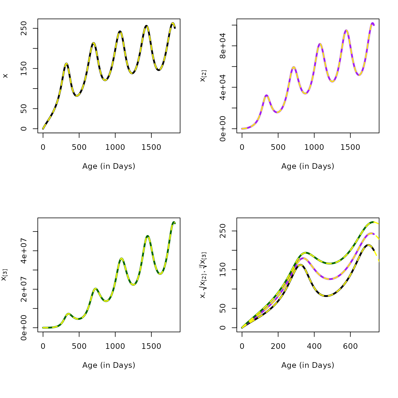

Derivation for $dx/da$

In Dynamics, we present an equation for $z_\tau(\alpha,a),$ the density function for infections of age $\alpha$ in a host cohort of age $a$ born on day $\tau$. The dynamics of $z(\alpha,a)$ are described by the following:

$$\begin{equation} \tag{1} \frac{\partial z}{\partial a} + \frac{\partial z}{\partial \alpha} = - r z \end{equation}$$

with the boundary condition:

$$z_\tau(0,a) = h_\tau(a)$$

and its solutions are:

$$z_\tau(\alpha,a) = h_\tau(a-\alpha) e^{-r \alpha}$$

In MoI, we defined the distribution function for the MoI:

$$M_\tau(a) \sim f_M(\zeta; a, \tau) = \mbox{Pois}(m_\tau(a))$$

and we showed that the mean MoI, $m_\tau(a)$ is:

$$\begin{equation} m_\tau(a) = \int_0^a z_\tau(\alpha, a) d \alpha \end{equation}$$

In AoI, we defined a probability density function for the AoI:

$$A_\tau(a) \sim f_A(\alpha; a, \tau) = \frac{z_\tau(\alpha,a)}{m_\tau(a)}$$

Here, we derive an equation for $$\frac{dx}{da} = \frac{d\left<A\right>}{da}$$

We start by multiplying Eq. 1 by $\alpha$ and integrating with respect to $\alpha$:

$$\begin{equation} \int_0^a \alpha \frac{\partial z(\alpha, a)}{\partial a} d \alpha + \int_0^a \alpha \frac{\partial z(\alpha, a)}{\partial \alpha} d\alpha = - r \int_0^a \alpha z(\alpha, a) d\alpha, \end{equation}$$

By its definition,

$$\int_0^a \alpha z(\alpha, a) d\alpha = \left<A \right> m$$

So we can simplify a bit:

$$\begin{equation} \tag{2} \frac{\partial \left<A \right>m}{\partial a} d \alpha + \int_0^a \alpha \partial z = - r \left<A \right> m \end{equation}$$

On the RHS of Eq. 2, the first term can be rewritten:

$$\begin{equation} \frac{\partial \left<A \right> m}{\partial a}= m \frac{\partial \left<A \right>}{\partial a} + \left<A \right> \frac{\partial m}{\partial a} \end{equation}$$

On the RHS of Eq. 2, the second term can be rewritten by integrating by parts:

$$\begin{equation} \int_0^a \alpha \partial z = \alpha z(a,\alpha) \big|_{\alpha = a} - \alpha z(a,\alpha) \big|_{\alpha = 0} - \int_0^a z d\alpha \end{equation}$$

which simplifies to:

$$\begin{equation} \int_0^a \alpha \partial z = a h_d(0)e^{-ra} - m \end{equation}$$

Substituting, we get:

$$\begin{equation} m \frac{\partial \left<A \right>}{\partial a} + \left<A \right> \frac{\partial m}{\partial a} + a h_d(0)e^{-ra} - m = - r \left<A \right> m \end{equation}$$

We divide through by $m$ and rearrange to get:

$$\begin{equation} \frac{\partial \left<A \right>}{\partial a} = - \frac{\left< A \right>}{m} \frac{\partial m}{\partial a} - \frac{a}{m} h_d(0)e^{-ra} + 1 - r \left<A \right> \end{equation}$$

We substitute $dm/da = h - rm$ and simplify:

$$\begin{equation} \frac{\partial \left<A \right>}{\partial a} = - \frac{\left< A \right>}{m} (h - rm) - \frac{a}{m} h_d(0)e^{-ra} + 1 - r \left<A \right> \end{equation}$$

and after rearranging terms and cancelling:

$$\begin{equation} \frac{\partial \left<A \right>}{\partial a} = 1 - h \frac{\left< A \right>}{m} - \frac{a}{m} h_d(0)e^{-ra} \end{equation}$$

or since we are letting $x = \left< A \right>$ $$\begin{equation} \frac{d x}{d a} = 1 - \frac{h}{m} x - \frac{a}{m} h_d(0)e^{-ra} \end{equation}$$

I can’t remember why that last term goes away

Noting that: $$\begin{equation} \lim_{m\rightarrow 0} \frac{A}{m} = \lim_{m\rightarrow 0} \frac{a}{m} = 1 \end{equation}$$

Derivation for $dx_n/da$

To derive a tracking equation for $\left<A^n \right>$, we start as before but multiply by $\alpha^n$ to get:

$$\begin{equation} \int_0^a \alpha^n \frac{\partial z}{\partial a} \partial \alpha + \int_0^a \alpha^n \frac{\partial z}{\partial \alpha} \partial \alpha = \int_0^a - r \alpha^n z \partial \alpha \end{equation}$$ which we can rewrite as: $$\begin{equation} \frac{\partial \left<A^n \right> m}{\partial a} + \int_0^a \alpha^n \partial x = - r \left<A^n\right> m \end{equation}$$

Integrating the middle term by parts,

$$\begin{equation} \int_0^a \alpha^n \partial z = \alpha^n z(a,\alpha) \big|_{\alpha = 0}^{a} - n \int_0^a \alpha^{n-1} z d\alpha \end{equation}$$

so we can rearrange this to get Eq.~$\ref{dAnda}$. Once again, we are concerned with the limits as $m$ becomes small:

$$\begin{equation} \lim_{m\rightarrow 0} \frac{A}{m} = \lim_{m\rightarrow 0} \frac{a}{m} = 1 \end{equation}$$