Scaling

ramp.work has functions to compute scaling relationships: how do various measures of malaria change across the spectrum of malaria transmission intensity?

This vignette explains the functions in ramp.work that:

compute scaling relationships
visualize scaling relationships

A longer introduction to scaling can be found in SimBA.

xds_scaling enables Metric Conversion

Pseudocode

Suppose that we have defined a model family: we modify a single parameter that changes the mean intensity of exposure or transmission, but we leave the rest of the parameters fixed.

To study the relationship between exposure and malaria outcomes, we might vary the mean annual EIR.
To study the relationship between mosquito density and outcomes, we might vary the average annual emergence rate. $\Lambda.$

To compute scaling relationships in systems with a seasonal forcing pattern, we will need to compute the stable orbits and link the outputs to the average annual values.

The function xds_scaling handles this task.

create a mesh of values for mean forcing, either
- the mean daily EIR, $\bar E.$
- the mean daily emergence rate for adult mosquitoes, $\bar \Lambda$ or Lambda.
for each mesh value:
- compute and store the stable orbits for important terms
- compute and store the mean values of the stable orbits

Example

Load the required packages:

library(ramp.xds)
library(ramp.work)

Set up a model forced by the EIR with a seasonal pattern, and we use ramp.xds::show_season to see the pattern:

Spar  <- makepar_F_sin(bottom = 0.2, pw=2)
model <- xds_setup_eir(eir = 1/365, season_par = Spar)
model <- xds_solve(model)
show_season(model)

The function xds_scaling computes and stores the values:

xds_scaling$scaling stores the average annual values by name
xds_scaling$scaling$stable_orbits stores the stable orbits

xds_scaling(model) -> model
names(model$scaling)

## [1] "aeir"          "eir"           "pr"            "ni"           
## [5] "stable_orbits"

A plot_eirpr plot the PfPR as a function of the average annual PfEIR on a semi-log plot. A function add_eirpr_orbits adds the stable orbits for an indexed subset. We use the virisLite::turbo color scheme so it is easy to relate the orbit and the mean value.

library(viridisLite)
xds_plot_eirpr(model)
ix_subset = c(9, 13, 17, 21)
add_eirpr_orbits(ix_subset, model, clrs = turbo(25))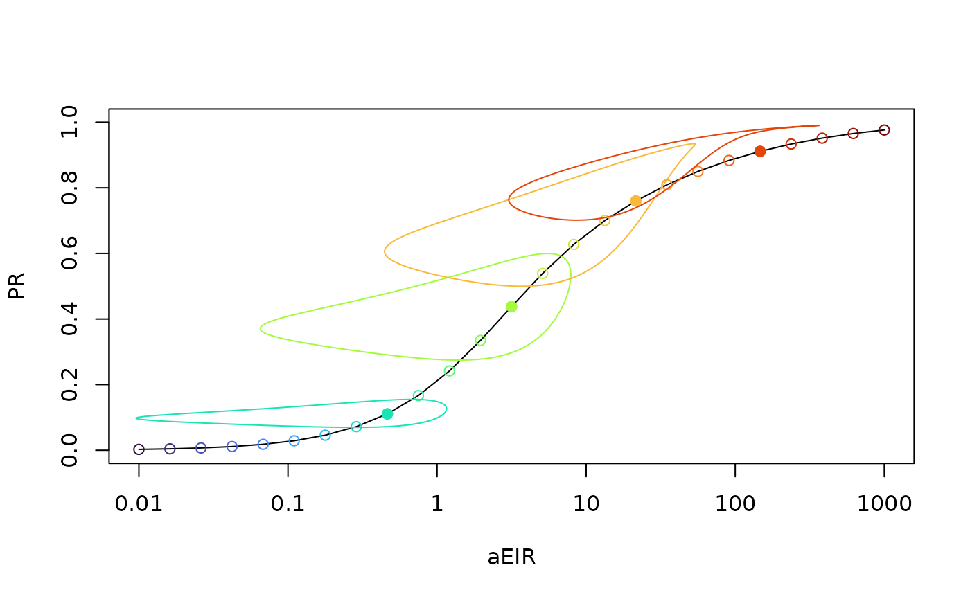

Notes

xds_scaling dispatches on xds_obj$forced_by, which is set up either by xds_setup_eir or by the make_L_obj_trivial.
The function xds_scaling.eir() creates a mesh over logged values of on an even mesh for values of log(aEIR) running from $10^{-2}$ up to $10^{3}.$
The function xds_scaling.Lambda() computes a creates a crude mesh. The first step is to compute an approximate pseudo-threshold value $L.$ The initial mesh looks has five values $c(L/100, L/5, L, 5L, 100L).$ Subsequent values are identified by picking a new value in the interval that has the largest change in PfPR. After adding the new value, the

Compute Scaling Relationships for Malaria Metrics

October 13, 2025

Pseudocode

Example

Notes