A constructor for seasonality functions drawn from a generalized
family involving trigonometric functions is returned by
make_function.sin with the associated
makepar_F_sin that returns functions of the form: \[F_S(t) = c\left(1 + \epsilon + \sin\left(\frac{2
\pi (t-\tau)}P\right)\right)^q\]
\(c\) or
normis a normalizing constant\(\tau\) or
phasesets the timing of the peak\(\epsilon \geq 0\) or
bottomis a shape parameter: increasing the values of \(\epsilon\) reduces the variance\(q \geq 0\) or
pwis a shape parameter\(P \geq 0\) or
periodsets the period of the function
p1 = makepar_F_sin()
S1 <- make_function(p1)
The default normalizing constant is equal to the period (by default, \(365\)) so that if \(S\) is multiplied by some other constant, \(m,\) the average daily value of the function over a year is \(1.\)
integrate(S1, 0, 365)$val## [1] 365
tt <- seq(0, 3*365, by=5)
plot(tt, S1(tt), type ="l", xlab = "Time (in Days)", ylab = expression(S(t)))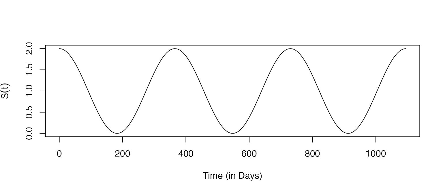
p2 = makepar_F_sin(phase=120)
S2 <- make_function(p2)
plot(tt, S1(tt), type ="l", xlab = "Time (in Days)", ylab = expression(S(t)))
lines(tt, S2(tt), col = "blue")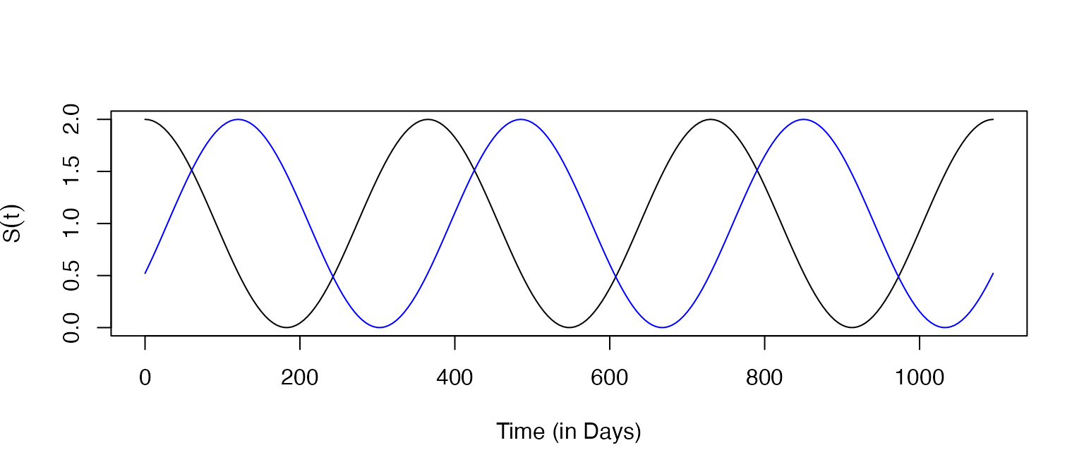
The function can return a vector of \(N\) functions, each one configured as if \(N=1\)
p3 = makepar_F_sin(phase = c(0,120), N=2)
S3 <- make_function(p3)
s3 <- S3(tt)
plot(tt, s3[1,], type ="l", xlab = "Time (in Days)", ylab = expression(S(t)))
lines(tt, S1(tt), col = "yellow", lty=2)
lines(tt, s3[2,], col = "blue")
lines(tt, S2(tt), col = "orange", lty=2)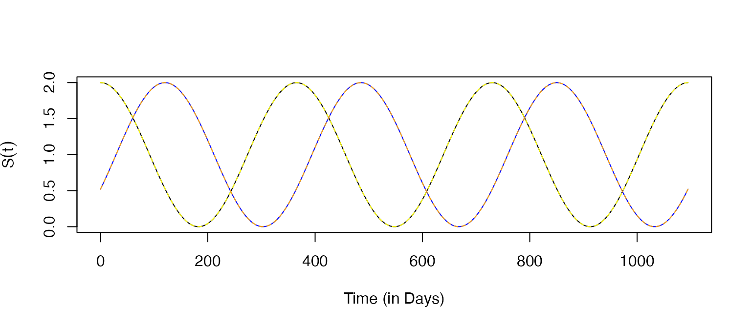
p4 <- makepar_F_sin(bottom=.5)
p5 <- makepar_F_sin(bottom=2)
p6 <- makepar_F_sin(pw=3)
p7 <- makepar_F_sin(pw=6)
S4 <- make_function(p4)
S5 <- make_function(p5)
S6 <- make_function(p6)
S7 <- make_function(p7)
The shape parameters make it easy to configure a seasonality function with a range of features:
clrs = turbo(7)
plot(tt, S7(tt), type ="n", xlab = "Time (in Days)", ylab = expression(S(t)))
lines(tt, S1(tt), col = clrs[1])
lines(tt, S4(tt), col = clrs[2])
lines(tt, S5(tt), col = clrs[3])
lines(tt, S6(tt), col = clrs[5])
lines(tt, S7(tt), col = clrs[7])
text(1000, 3.5, expression(p==6), col=clrs[7])
text(1000, 3, expression(p==3), col=clrs[5])
text(1000, 2.5, expression(epsilon==0.5), col=clrs[2])
text(1000, 2, expression(epsilon==2), col=clrs[3])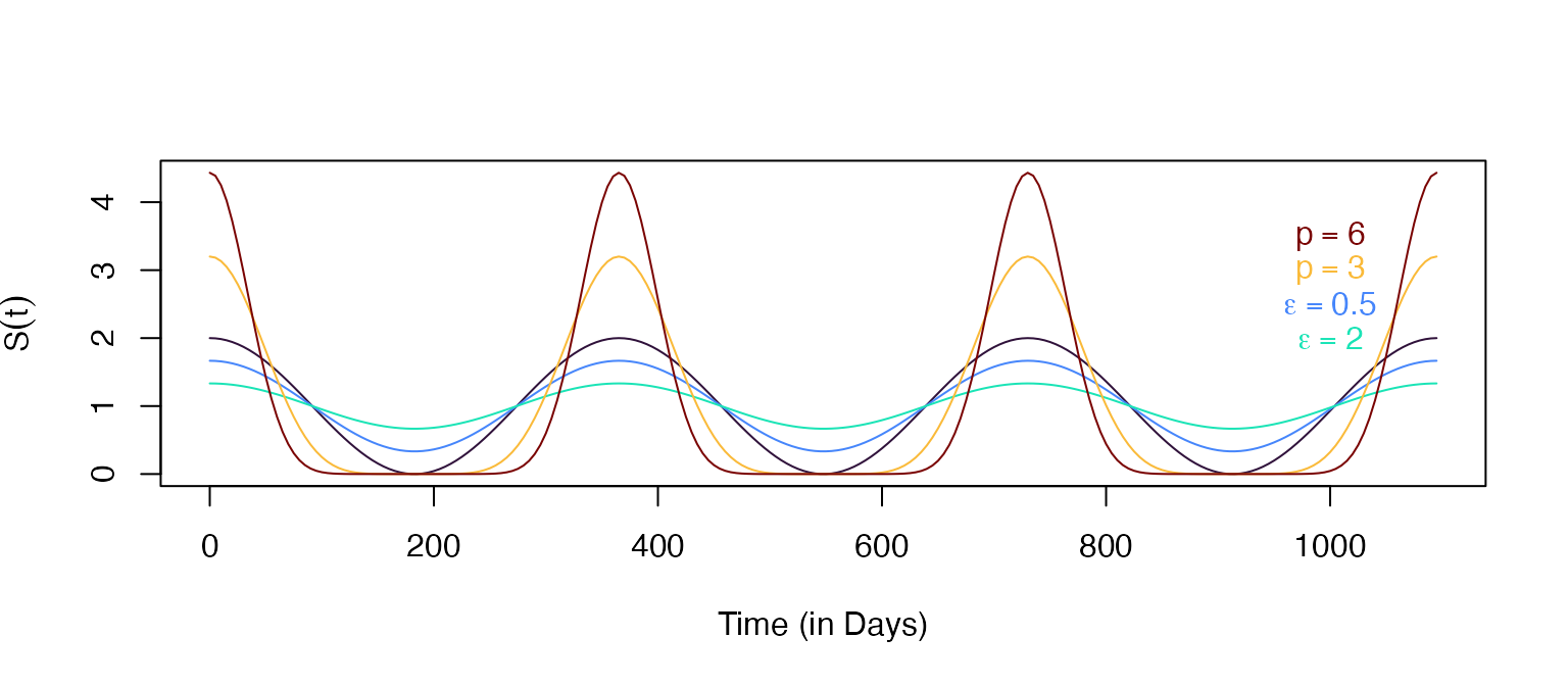
Multiple Periods
p1 <- makepar_F_sin()
p2 <- makepar_F_sin(period=1, bottom=1)
p12 <- makepar_F_product(p1, p2)
S2 <- make_function(p12)
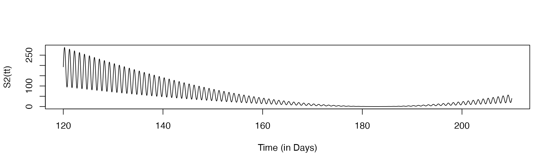
This plots the function over a stretch of values:
integrate(S2, 0, 365, rel.tol=1e-3)$value## [1] 133225
p12a<- makepar_F_product(p1, p2, P=365, tol = 1e-3)
S2a <- make_function(p12a)
integrate(S2a, 0, 365, rel.tol=1e-3)$value
## [1] 365