Ross-Macdonald Mosquito Infection Dynamics

library(ramp.dts)
#devtools::load_all()

In this vignette, we present a model for the dynamics of malaria infection in adult mosquito populations. We call it a Ross-Macdonald model because it makes the same basic assumptions as the model that Macdonald analyzed in 1952. While that model was developed using differential equations, the equations we describe herein are difference equations.

We begin by discrete-time model in a simple population, with one patch, and then we present the equations for the multi-patch model.

In a Single Patch

We define several variables describing adult female mosquitoes. Let \(M_t\) denote the total density of uninfected mosquitoes at time \(t.\) We assume that mosquitoes emerge from aquatic habitats at the rate \(\Lambda_t\) and that a proportion of mosquitoes, \(p\), survives each day. The total density of mosquitoes is described by an equation:

\[M_{t+1} = \Lambda_t + p M_t\]

We let \(f\) denote the proportion of mosquitoes that blood feeds each day, and let \(P_t\) denote the density of parous mosquitoes:

\[P_{t+1} = f(M_t - P_t) + p P_t\]

To model the infection process we need two additional parameters:

\(q\) - the proportion of blood meals that are taken on humans
\(\kappa_t\) - fraction of human blood meals that infect the mosquito

Let \(U\) denote the density of uninfected mosquitoes:

\[U_{t+1} = \Lambda_t + p e^{-f q \kappa_t} U_t \] Let \(Y_{i,t}\) denote a the density of cohorts of infected mosquitoes infected \(i\) days ago:

\[Y_{1, t+1} = p (1-e^{-f q \kappa_t}) U_t \] We let \(\tau\) denote the oldest cohort of infected mosquitoes that we would wish to track. For mosquitoes infected more than 1 day ago, we let \(G_i\) be the fraction that becomes infectious the next day. If we modeled the EIP with a fixed delay, then \(G_i = 1\) for \(i < \tau\), and \(G_\tau = 1\). Mosquitoes would become infectious on day \(\tau+1.\)

\[Y_{i+1, t+1} = p \left(1-G_i \right) Y_{i, t} \]

and

\[Y_{\tau, t+1} = p \left(1-G_{\tau-1} \right) Y_{\tau-1, t} + p \left(1-G_\tau \right) Y_{\tau, t}\]

\(Z_t\) denote the density of infectious mosquitoes at time \(t\)

\[Z_{t+1} = \sum_i p G_i Y_i + p Z_t\]

As we have defined our variables, one of them is not necessary, since

\[U = M- \sum_i Y_i - Z\]

The Multi-Patch Model

In a model with \(n\) patches, the model is defined as before, but now we let \(M_t,\) \(P_t,\) \(U_t\), and \(Z_t\) be vectors of length \(p,\) and we let \(G\) be a vector of length \(\tau,\) (where \(G_1 = 0\)). We let \(Y_t\) denote a \(p \times \tau\) matrix, where each row is a cohort of mosquitoes, and where column represents the mosquitoes in a location. We let \(Y_{i,t}\) denote the \(i^{th}\) cohort:

Now, we also need to define mosquito movement. We let \(\sigma\) denote a vector describing the proportion of mosquitoes that emigrates from each patch, and let \(\cal K\) denote a matrix describing the fraction of emigrating mosquitoes that end up in every other patch, where \[\mbox{diag}\; {\cal K} = 0.\] and where the columns sum up to a number that is less than or equal to one, where the gap represents mortality occurring during dispersal.

We let \(\Omega\) denote the demographic matrix where:

\[\Omega = \mbox{diag}\left( p \left( 1-\sigma \right) \right) + \mbox{diag}\left( p \sigma \right) \cdot {\cal K} \] Now the dynamics are very similar:

\[ \begin{array}{rl} M_{t+1} &= \Lambda_t + \Omega \cdot M_t \\ P_{t+1} &= f (M_t - P_t) + \Omega \cdot P_t \\ \hline U_{t+1} &= \Lambda_t + \Omega \cdot \left(e^{-fq\kappa_t} U_t \right) \\ Y_{1, t+1} &= \Omega \cdot \left(\left(1-e^{-fq\kappa_t}\right) U_t \right) \\ Y_{i+1, t+1} &= \Omega \cdot Y_{i,t} \left(1-G_i \right) \\ Y_{\tau, t+1} &= \Omega \cdot \left( Y_{\tau-1, t}\;\left(1-G_{\tau-1} \right) \right) + \Omega \cdot \left( Y_{\tau, t} \; \left(1-G_\tau \right) \right) \\ Z_{t+1} &= \Omega \cdot \left(Y_t \cdot \mbox{diag}(G) \right)+ \Omega \cdot Z_t \\ \end{array} \]

Implementation Notes:

In the implementation, we could choose models where the EIP is distributed over some period but where the fraction maturing after time \(\tau\) is continuous. We have chosen a rotating index to track age of infection cohorts in the matrix \(Y;\) using modulo arithmetic, each columns tracks a single cohort for \(\tau\) days. On the \(\tau +1\) day, the column is added to the one before, and then we compute \(Y_{1,t}.\) The computation thus does this:

\[\begin{array}{rl} M_{t+1} &= \Lambda_t + \Omega \cdot M_t \\ P_{t+1} &= f(M_t-P_t) + \Omega \cdot P_t \\ \hline U_{t+1} &= \Lambda_t + \Omega \cdot \left(e^{-fq\kappa_t} U_t \right) \\ Y_{t+1} &= \Omega \cdot \left(Y_{i, t} \cdot \mbox{diag} \left(1-G \right) \right) \\ Z_{t+1} &= \Omega \cdot \left( Y_t \cdot \mbox{diag}\; G \right)+ \Omega \cdot Z_t \\ \end{array}\]

Noting that in the modulo arithmetic, \(\tau+1 = 1\), we get:

\[ \begin{array}{rl} Y_{\tau, t+1} &= Y_{\tau, t+1} + Y_{\tau+1, t} \\ Y_{1, t+1} &= \Omega \cdot \left(\left(1-e^{-fq\kappa_t}\right) U_t \right) \\ \end{array} \]

Verification

We can verify our model by solving for steady states.

\[\bar M = \Lambda \cdot (1-\Omega)^{-1}\]

\[\bar P = f \bar M \cdot (1-\Omega+ \mbox{diag}\;f )^{-1}\]

\[\bar U = \Lambda \cdot (1-\Omega \cdot \mbox{diag}\; e^{-fq\kappa})^{-1}\]

\[\bar Y_1 = \Omega \cdot \left( 1- e^{-fq\kappa}\right) \cdot \bar U\] For \(1 < i < \tau,\) we get a recursive relationship:

\[\bar Y_{i+1} = \Omega \cdot \; \bar Y_i (1-G_i) \] and for \(Y_{\tau},\) we get:

\[\bar Y_{\tau} = \Omega \cdot \left( \mbox{diag} \left(1-G\right) \right) \bar Y_{\tau-1} \cdot \left(1 - \Omega \left (1-G_\tau \right) \right)^{-1}\] and

\[\bar Z = \Omega \cdot G \cdot Y \left( 1- \Omega\right)^{-1}\]

Demo

devtools::load_all()

rm1 <- dts_setup(Xname = "trace")

dts_solve(rm1, Tmax=200) -> rm1

dts_steady(rm1) -> rm1

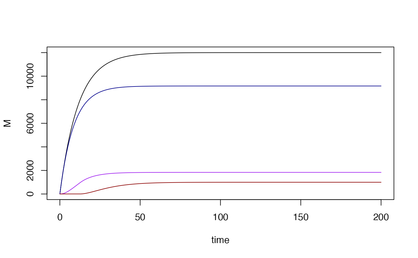
with(rm1$outputs$orbits$MYZ[[1]], {
  plot(time, M, type = "l") 
  lines(time, U, col = "darkblue") 
  lines(time, Y, col = "purple") 
  lines(time, Z, col = "darkred") 
})

dts_plot_YZ(rm1)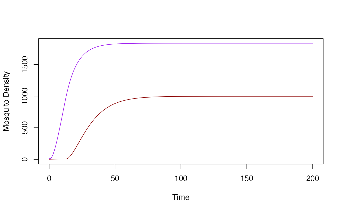

compute_MYZ_equil = function(pars, Lambda, kappa, i=1){
  Omega = make_Omega(0, pars$MYZpar[[i]])
  with(pars$MYZpar[[i]],{

    Mbar <-  Lambda/(1-p) 
    Pbar <- f*Mbar/(1 - p + f)
    Ubar <- Lambda/(1-p*exp(-f*q*kappa))
    
    Y1 <- Omega*(1-exp(-f*q*kappa))*Ubar 
    Yi = Y1
    Y = Yi
    for(i in 2:(max_eip-1)){
      Yi <- Omega*Yi*(1-G[i])
      Y = Y+Yi
    }
    Yn <- Omega*Yi
    Y = Y + Yn
    Zbar <- Omega*Yn/(1-p) 
    return(c(M = Mbar, P=Pbar, U=Ubar, Y=Y, Z= Zbar)) 
})}

compute_MYZ_equil(rm1, 1000, .1) 
#>          M          P          U          Y          Z 
#> 12000.0000  9391.3043  9166.7797  1835.9391   997.2812

c(
M = tail(rm1$outputs$orbits$MYZ[[1]]$M, 1), 
P = tail(rm1$outputs$orbits$MYZ[[1]]$P, 1), 
U = tail(rm1$outputs$orbits$MYZ[[1]]$U, 1),
Y = tail(rm1$outputs$orbits$MYZ[[1]]$Y, 1),
Z = tail(rm1$outputs$orbits$MYZ[[1]]$Z, 1)
)
#>          M          P          U          Y          Z 
#> 11999.9997  9391.3040  9166.7797  1835.9391   997.2808

rm10 <- dts_setup(Xname = "trace", nPatches = 10, membership = 1:10)
rm10$Lpar[[1]]$scale = 1.5^c(1:10)

dts_solve(rm10, Tmax=200) -> rm10

with(rm10$outputs$orbits$MYZ[[1]], {
  plot(time, M[,10], type = "l")
  for(i in 2:10)
    lines(time, M[,i]) 
#  lines(time, U, col = "darkblue") 
#  lines(time, Y, col = "purple") 
#  lines(time, Z, col = "darkred") 
})

Discrete-Time Dynamics

In a Single Patch

The Multi-Patch Model

Implementation Notes:

Verification

Demo