IRS

library(ramp.xds)
library(ramp.control)
library(MASS)
library(deSolve)
library(viridisLite)

#devtools::load_all()

ramp.control handles IRS in a flexible way. Four methods are defined; not all of them need to get used.

The irs model object

irs

$spray_mod
$effects_mod
$coverage_mod
coverage
$ef_sz_mod
- [[1]] - for species 1
- …

For the xds model object called model:

VectorControl::IRS
- SprayHouses – a function to model mass distribution of nets and/or coverage dispatched by class(model$irs$spray_mod)
- IRSEffects – modify mosquito behavioral parameters, including search weights dispatched by class(model$irs$effects_mod)
VectorControl::IRSEffectSizes
- IRSCoverage – compute IRS coverage dispatched by class(model$irs$coverage_mod)
- After evaluating IRSCoverage, values are stored at model$irs$coverage
- IRSEffectSizes – compute IRS effect sizes dispatched by class(model$irs$ef_sz_mod[[s]]) (for the $s^{th}$ species)

Coverage

IRS is usually done through a malaria program, so a large number of houses are sprayed in a short period of time. One measure of coverage is the fraction of houses sprayed, $C$, but since the potency of the insecticide wanes over time, we define coverage as the product of the fraction of houses sprayed and potency, $P(t)$. It is an operational measure that we can define without thinking much about mosquito behaviors. Coverage is thus independent of mosquito species.

To model coverage, we developed the sharkfin functions in ramp.xds, the product of two sigmoidal functions – one ramping up and the other down with different shapes. With this sharkfin function, coverage increases over 20 days from zero up to 90%, reaching 50% of the maximum on day 50. Potency wanes, reaching 50% on day 230, 180 days after the spray round.

irs_par <- makepar_F_sharkfin(D=50, uk=1/3, L=180, mx=.9)
Fsf <- make_function(irs_par)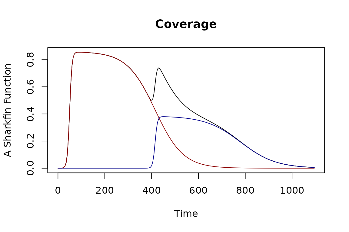

model <- xds_setup(MYname = "SI", Loptions = list(Lambda=40, season_par=makepar_F_sin()))
model <- xds_solve(model, 2000)
model <- last_to_inits(model)
model <- xds_solve(model, 1100)
xds_plot_EIR(model)

model <- setup_irs(model, coverage_name = "func", coverage_opts=list(trend_par = irs_par, mx=1), effect_sizes_name = "simple")

show_irs_contact(tt, model)

model <- xds_solve(model, 1100)
xds_plot_EIR(model)

Effect Sizes

The effects of IRS and effect sizes are related to realized coverage, $\phi$: to have an effect, the mosquito must come into contact with the IRS, and the behaviors of different mosquito species affect how often they will rest on a sprayed surface. We call this contact parameter zap. Realized coverage is the product of coverage and the contact parameter.

Models for effect sizes translate realized coverage into changes in the values of mosquito bionomic parameters. In a simple model, called simple, mortality changes from baseline $g$ assuming that there is addtional mortality every time a mosquito blood feeds on a human and makes contact with a sprayed surface:

\[ g \rightarrow g + f q \phi\]

The effect sizes is the ratio of the modified mortality rate over baseline:

\[ \frac{g + fq\phi}{g} = 1 + \phi \frac{fq}{g}.\] The effect size is computed relative to a baseline bionomic parameter set, and it is returned by models for independent effect sizes. The effect size is returned, rather than the modified parameters, in case multiple modes of control are operating. Later, the baseline is modified by control by taking the product of the baseline and all the independent effect sizes.

Building Indoor Residual Spraying Models

Coverage

Effect Sizes